replaced http://scicomp.stackexchange.com/ with https://scicomp.stackexchange.com/
Source Link

I am interested in implementing an moving mesh for an advection-diffusion problem. Adaptive Moving Mesh Methods gives a good example of how to do this for Burger's equation in 1D using finite-difference. Would someone be able to offer a worked example on solving the 1D advection-diffusion equation using finite-difference with a moving mesh?

For example, in conservative form the equation is,

$$ u_t = (a(x)u + du_x)_x $$

where $a(x)$ is the velocity (a function of space). The initial conditions $u(0,x)$ could specify (for example) a flow species moving from left to right (e.g. along a pipe) where the initial condition has a sharp gradient.

How should the equidistribution problem for the moving mesh be solved (possibly with De Boor's algorithm or other approach)? I wish to implement this myself in Python so if your answer can be readily translated into code all the better!


Old question prior to bounty

  1. What are the basic approaches for generating an adaptive mesh based on properties of the system? Should I use flux as a measure of where the gradients are large?
  2. Because I seek an iterative (time sweep) solution. I imagine it is important to interpolate from the old grid to the new grid, what is the usual approach?
  3. I would be really interested to see a worked example for a simple problem (like the advection equation).

A bit of background about the specifics of the problem. I am simulating a 1D coupled system of equation,

$ \frac{\partial u}{\partial t} = a_u\frac{\partial^2 u}{\partial x^2} + b_u\frac{\partial u}{\partial x} + f_u(x,u,v,w) \\ \frac{\partial v}{\partial t} = a_v\frac{\partial^2 v}{\partial x^2} + b_v\frac{\partial v}{\partial x} + f_v(x,u,v,w) \\ \frac{\partial w}{\partial t} = a_u\frac{\partial u}{\partial x} +a_v\frac{\partial v}{\partial x} + f_w(x,u,v,w) \\ $

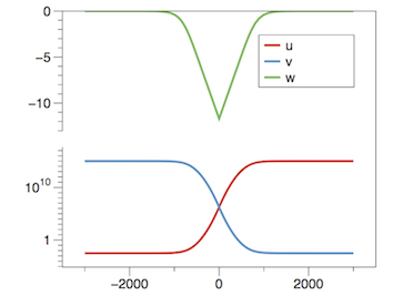
The set of equations describe a two species advection-diffusion problem where the third equation couples to the other two. The solution change rapidly near the centre of my grid, see below (these are illustration not calculations),
Example solutions

Notice that log scale on the lower graph, the solutions for $u$ and $v$ vary over orders of magnitude. On the upper graph ($w$) there is a discontinuity at the centre. I am solving the above system with an adaptive upwind where the discretization can adapt from central to upwind dominated depending on local value of Péclet number. I am solving the system implicitly with trapezoidal integration in time ("Crank-Nicolson").

I am interested in applying an adaptive grid to this problem. I think it is important because otherwise details of the shape peak (the $w$) parameter could be lost. Unlike this questionquestion, I would like to apply, a hopefully simply, algorithm for mesh generation.

As this is an advection-diffusion problem, one could imagine an adaptive mesh scheme based on the fluxes of $u$ and $v$ at the cell boundaries. As this would indicate where the value is changing rapidly. The peak of the $w$ also corresponds to the where the flux are the largest.

I am interested in implementing an moving mesh for an advection-diffusion problem. Adaptive Moving Mesh Methods gives a good example of how to do this for Burger's equation in 1D using finite-difference. Would someone be able to offer a worked example on solving the 1D advection-diffusion equation using finite-difference with a moving mesh?

For example, in conservative form the equation is,

$$ u_t = (a(x)u + du_x)_x $$

where $a(x)$ is the velocity (a function of space). The initial conditions $u(0,x)$ could specify (for example) a flow species moving from left to right (e.g. along a pipe) where the initial condition has a sharp gradient.

How should the equidistribution problem for the moving mesh be solved (possibly with De Boor's algorithm or other approach)? I wish to implement this myself in Python so if your answer can be readily translated into code all the better!


Old question prior to bounty

  1. What are the basic approaches for generating an adaptive mesh based on properties of the system? Should I use flux as a measure of where the gradients are large?
  2. Because I seek an iterative (time sweep) solution. I imagine it is important to interpolate from the old grid to the new grid, what is the usual approach?
  3. I would be really interested to see a worked example for a simple problem (like the advection equation).

A bit of background about the specifics of the problem. I am simulating a 1D coupled system of equation,

$ \frac{\partial u}{\partial t} = a_u\frac{\partial^2 u}{\partial x^2} + b_u\frac{\partial u}{\partial x} + f_u(x,u,v,w) \\ \frac{\partial v}{\partial t} = a_v\frac{\partial^2 v}{\partial x^2} + b_v\frac{\partial v}{\partial x} + f_v(x,u,v,w) \\ \frac{\partial w}{\partial t} = a_u\frac{\partial u}{\partial x} +a_v\frac{\partial v}{\partial x} + f_w(x,u,v,w) \\ $

The set of equations describe a two species advection-diffusion problem where the third equation couples to the other two. The solution change rapidly near the centre of my grid, see below (these are illustration not calculations),

Example solutions

Notice that log scale on the lower graph, the solutions for $u$ and $v$ vary over orders of magnitude. On the upper graph ($w$) there is a discontinuity at the centre. I am solving the above system with an adaptive upwind where the discretization can adapt from central to upwind dominated depending on local value of Péclet number. I am solving the system implicitly with trapezoidal integration in time ("Crank-Nicolson").

I am interested in applying an adaptive grid to this problem. I think it is important because otherwise details of the shape peak (the $w$) parameter could be lost. Unlike this question, I would like to apply, a hopefully simply, algorithm for mesh generation.

As this is an advection-diffusion problem, one could imagine an adaptive mesh scheme based on the fluxes of $u$ and $v$ at the cell boundaries. As this would indicate where the value is changing rapidly. The peak of the $w$ also corresponds to the where the flux are the largest.

Notice removed Canonical answer required by CommunityBot
Bounty Ended with no winning answer by CommunityBot
More detail in the question.
Source Link
boyfarrell
  • 5.4k
  • 3
  • 35
  • 67

I am interested in implementing an moving mesh for an advection-diffusion problem. Adaptive Moving Mesh Methods gives a good example of how to do this for Burger's equation in 1D using finite-difference. Would someone be able to offer a worked example on solving the 1D advection-diffusion equation using finite-difference with a moving mesh?

For example, in conservative form the equation is,

$$ u_t = (a(x)u + du_x)_x $$

where $a(x)$ is the velocity (a function of space). The initial conditions $u(0,x)$ could specify (for example) a flow species moving from left to right (e.g. along a pipe) where the initial condition has a sharp gradient.

How should the equidistribution problem for the moving mesh be solved (possibly with De Boor's algorithm or other approach)? I wish to implement this myself in Python so if your answer can be readily translated into code all the better!


Old question prior to bounty

  1. What are the basic approaches for generating an adaptive mesh based on properties of the system? Should I use flux as a measure of where the gradients are large?
  2. Because I seek an iterative (time sweep) solution. I imagine it is important to interpolate from the old grid to the new grid, what is the usual approach?
  3. I would be really interested to see a worked example for a simple problem (like the advection equation).

A bit of background about the specifics of the problem. I am simulating a 1D coupled system of equation,

$ \frac{\partial u}{\partial t} = a_u\frac{\partial^2 u}{\partial x^2} + b_u\frac{\partial u}{\partial x} + f_u(x,u,v,w) \\ \frac{\partial v}{\partial t} = a_v\frac{\partial^2 v}{\partial x^2} + b_v\frac{\partial v}{\partial x} + f_v(x,u,v,w) \\ \frac{\partial w}{\partial t} = a_u\frac{\partial u}{\partial x} +a_v\frac{\partial v}{\partial x} + f_w(x,u,v,w) \\ $

The set of equations describe a two species advection-diffusion problem where the third equation couples to the other two. The solution change rapidly near the centre of my grid, see below (these are illustration not calculations),

Example solutions

Notice that log scale on the lower graph, the solutions for $u$ and $v$ vary over orders of magnitude. On the upper graph ($w$) there is a discontinuity at the centre. I am solving the above system with an adaptive upwind where the discretization can adapt from central to upwind dominated depending on local value of Péclet number. I am solving the system implicitly with trapezoidal integration in time ("Crank-Nicolson").

I am interested in applying an adaptive grid to this problem. I think it is important because otherwise details of the shape peak (the $w$) parameter could be lost. Unlike this question, I would like to apply, a hopefully simply, algorithm for mesh generation.

As this is an advection-diffusion problem, one could imagine an adaptive mesh scheme based on the fluxes of $u$ and $v$ at the cell boundaries. As this would indicate where the value is changing rapidly. The peak of the $w$ also corresponds to the where the flux are the largest.

I am interested in implementing an moving mesh for an advection-diffusion problem. Adaptive Moving Mesh Methods gives a good example of how to do this for Burger's equation in 1D using finite-difference. Would someone be able to offer a worked example on solving the 1D advection-diffusion equation using finite-difference with a moving mesh?

For example, in conservative form the equation is,

$$ u_t = (a(x)u + du_x)_x $$

where $a(x)$ is the velocity (a function of space). The initial conditions $u(0,x)$ could specify (for example) a flow species moving from left to right (e.g. along a pipe) where the initial condition has a sharp gradient.

How should the equidistribution problem for the moving mesh be solved (possibly with De Boor's algorithm or other approach)? I wish to implement this myself in Python so if your answer can be readily translated into code all the better!


Old question prior to bounty

  1. What are the basic approaches for generating an adaptive mesh based on properties of the system? Should I use flux as a measure of where the gradients are large?
  2. Because I seek an iterative (time sweep) solution. I imagine it is important to interpolate from the old grid to the new grid, what is the usual approach?
  3. I would be really interested to see a worked example for a simple problem (like the advection equation).

A bit of background about the specifics of the problem. I am simulating a 1D coupled system of equation,

$ \frac{\partial u}{\partial t} = a_u\frac{\partial^2 u}{\partial x^2} + b_u\frac{\partial u}{\partial x} + f_u(x,u,v,w) \\ \frac{\partial v}{\partial t} = a_v\frac{\partial^2 v}{\partial x^2} + b_v\frac{\partial v}{\partial x} + f_v(x,u,v,w) \\ \frac{\partial w}{\partial t} = a_u\frac{\partial u}{\partial x} +a_v\frac{\partial v}{\partial x} + f_w(x,u,v,w) \\ $

The set of equations describe a two species advection-diffusion problem where the third equation couples to the other two. The solution change rapidly near the centre of my grid, see below (these are illustration not calculations),

Example solutions

Notice that log scale on the lower graph, the solutions for $u$ and $v$ vary over orders of magnitude. On the upper graph ($w$) there is a discontinuity at the centre. I am solving the above system with an adaptive upwind where the discretization can adapt from central to upwind dominated depending on local value of Péclet number. I am solving the system implicitly with trapezoidal integration in time ("Crank-Nicolson").

I am interested in applying an adaptive grid to this problem. I think it is important because otherwise details of the shape peak (the $w$) parameter could be lost. Unlike this question, I would like to apply, a hopefully simply, algorithm for mesh generation.

As this is an advection-diffusion problem, one could imagine an adaptive mesh scheme based on the fluxes of $u$ and $v$ at the cell boundaries. As this would indicate where the value is changing rapidly. The peak of the $w$ also corresponds to the where the flux are the largest.

Notice added Canonical answer required by boyfarrell
Bounty Started worth 100 reputation by boyfarrell
Edited for bounty.
Source Link
boyfarrell
  • 5.4k
  • 3
  • 35
  • 67

What are the basic principles behind generating an adaptivea moving mesh?

I am interested in implementing an moving mesh for an advection-diffusion problem. Adaptive Moving Mesh Methods gives a good example of how to do this for Burger's equation in 1D using finite-difference. Would someone be able to offer a worked example on solving the 1D advection-diffusion equation using finite-difference with a moving mesh?

For example, in conservative form the equation is,

$$ u_t = (a(x)u + du_x)_x $$

where $a(x)$ is the velocity (a function of space). The initial conditions $u(0,x)$ could specify (for example) a flow species moving from left to right (e.g. along a pipe) where the initial condition has a sharp gradient.


Old question prior to bounty

  1. What are the basic approaches for generating an adaptive mesh based on properties of the system? Should I use flux as a measure of where the gradients are large?
  2. Because I seek an iterative (time sweep) solution. I imagine it is important to interpolate from the old grid to the new grid, what is the usual approach?
  3. I would be really interested to see a worked example for a simple problem (like the advection equation).

A bit of background about the specifics of the problem. I am simulating a 1D coupled system of equation,

$ \frac{\partial u}{\partial t} = a_u\frac{\partial^2 u}{\partial x^2} + b_u\frac{\partial u}{\partial x} + f_u(x,u,v,w) \\ \frac{\partial v}{\partial t} = a_v\frac{\partial^2 v}{\partial x^2} + b_v\frac{\partial v}{\partial x} + f_v(x,u,v,w) \\ \frac{\partial w}{\partial t} = a_u\frac{\partial u}{\partial x} +a_v\frac{\partial v}{\partial x} + f_w(x,u,v,w) \\ $

The set of equations describe a two species advection-diffusion problem where the third equation couples to the other two. The solution change rapidly near the centre of my grid, see below (these are illustration not calculations),

Example solutions

Notice that log scale on the lower graph, the solutions for $u$ and $v$ vary over orders of magnitude. On the upper graph ($w$) there is a discontinuity at the centre. I am solving the above system with an adaptive upwind where the discretization can adapt from central to upwind dominated depending on local value of Péclet number. I am solving the system implicitly with trapezoidal integration in time ("Crank-Nicolson").

I am interested in applying an adaptive grid to this problem. I think it is important because otherwise details of the shape peak (the $w$) parameter could be lost. Unlike this question, I would like to apply, a hopefully simply, algorithm for mesh generation.

As this is an advection-diffusion problem, one could imagine an adaptive mesh scheme based on the fluxes of $u$ and $v$ at the cell boundaries. As this would indicate where the value is changing rapidly. The peak of the $w$ also corresponds to the where the flux are the largest.

What are the basic principles behind generating an adaptive mesh?

  1. What are the basic approaches for generating an adaptive mesh based on properties of the system? Should I use flux as a measure of where the gradients are large?
  2. Because I seek an iterative (time sweep) solution. I imagine it is important to interpolate from the old grid to the new grid, what is the usual approach?
  3. I would be really interested to see a worked example for a simple problem (like the advection equation).

A bit of background about the specifics of the problem. I am simulating a 1D coupled system of equation,

$ \frac{\partial u}{\partial t} = a_u\frac{\partial^2 u}{\partial x^2} + b_u\frac{\partial u}{\partial x} + f_u(x,u,v,w) \\ \frac{\partial v}{\partial t} = a_v\frac{\partial^2 v}{\partial x^2} + b_v\frac{\partial v}{\partial x} + f_v(x,u,v,w) \\ \frac{\partial w}{\partial t} = a_u\frac{\partial u}{\partial x} +a_v\frac{\partial v}{\partial x} + f_w(x,u,v,w) \\ $

The set of equations describe a two species advection-diffusion problem where the third equation couples to the other two. The solution change rapidly near the centre of my grid, see below (these are illustration not calculations),

Example solutions

Notice that log scale on the lower graph, the solutions for $u$ and $v$ vary over orders of magnitude. On the upper graph ($w$) there is a discontinuity at the centre. I am solving the above system with an adaptive upwind where the discretization can adapt from central to upwind dominated depending on local value of Péclet number. I am solving the system implicitly with trapezoidal integration in time ("Crank-Nicolson").

I am interested in applying an adaptive grid to this problem. I think it is important because otherwise details of the shape peak (the $w$) parameter could be lost. Unlike this question, I would like to apply, a hopefully simply, algorithm for mesh generation.

As this is an advection-diffusion problem, one could imagine an adaptive mesh scheme based on the fluxes of $u$ and $v$ at the cell boundaries. As this would indicate where the value is changing rapidly. The peak of the $w$ also corresponds to the where the flux are the largest.

What are the basic principles behind generating a moving mesh?

I am interested in implementing an moving mesh for an advection-diffusion problem. Adaptive Moving Mesh Methods gives a good example of how to do this for Burger's equation in 1D using finite-difference. Would someone be able to offer a worked example on solving the 1D advection-diffusion equation using finite-difference with a moving mesh?

For example, in conservative form the equation is,

$$ u_t = (a(x)u + du_x)_x $$

where $a(x)$ is the velocity (a function of space). The initial conditions $u(0,x)$ could specify (for example) a flow species moving from left to right (e.g. along a pipe) where the initial condition has a sharp gradient.


Old question prior to bounty

  1. What are the basic approaches for generating an adaptive mesh based on properties of the system? Should I use flux as a measure of where the gradients are large?
  2. Because I seek an iterative (time sweep) solution. I imagine it is important to interpolate from the old grid to the new grid, what is the usual approach?
  3. I would be really interested to see a worked example for a simple problem (like the advection equation).

A bit of background about the specifics of the problem. I am simulating a 1D coupled system of equation,

$ \frac{\partial u}{\partial t} = a_u\frac{\partial^2 u}{\partial x^2} + b_u\frac{\partial u}{\partial x} + f_u(x,u,v,w) \\ \frac{\partial v}{\partial t} = a_v\frac{\partial^2 v}{\partial x^2} + b_v\frac{\partial v}{\partial x} + f_v(x,u,v,w) \\ \frac{\partial w}{\partial t} = a_u\frac{\partial u}{\partial x} +a_v\frac{\partial v}{\partial x} + f_w(x,u,v,w) \\ $

The set of equations describe a two species advection-diffusion problem where the third equation couples to the other two. The solution change rapidly near the centre of my grid, see below (these are illustration not calculations),

Example solutions

Notice that log scale on the lower graph, the solutions for $u$ and $v$ vary over orders of magnitude. On the upper graph ($w$) there is a discontinuity at the centre. I am solving the above system with an adaptive upwind where the discretization can adapt from central to upwind dominated depending on local value of Péclet number. I am solving the system implicitly with trapezoidal integration in time ("Crank-Nicolson").

I am interested in applying an adaptive grid to this problem. I think it is important because otherwise details of the shape peak (the $w$) parameter could be lost. Unlike this question, I would like to apply, a hopefully simply, algorithm for mesh generation.

As this is an advection-diffusion problem, one could imagine an adaptive mesh scheme based on the fluxes of $u$ and $v$ at the cell boundaries. As this would indicate where the value is changing rapidly. The peak of the $w$ also corresponds to the where the flux are the largest.

added 30 characters in body
Source Link
boyfarrell
  • 5.4k
  • 3
  • 35
  • 67
Loading
Making the question clearer.
Source Link
boyfarrell
  • 5.4k
  • 3
  • 35
  • 67
Loading
Tweeted twitter.com/#!/StackSciComp/status/342869165633310720
Source Link
boyfarrell
  • 5.4k
  • 3
  • 35
  • 67
Loading