Interpolating a mathematical function using a Hermite Cubic Finite Element Space

Question

I have a Hermite Cubic Finite Element Space on a computer in the form of Matlab m-files. More specifically, I can evaluate four "shape functions" $N_1, N_2, N_3,$ and $N_4$, for which the following holds on the boundary of the "reference element" $K_R= [-1,1]$: \begin{align*} N_1(-1) = 1, N_1(1) = 0, N_1'(-1) = 0, N_1'(1) = 0,\\ N_2(-1) = 0, N_2(1) = 1, N_2'(-1) = 0, N_2'(1) = 0,\\ N_3(-1) = 0, N_3(1) = 0, N_3'(-1) = 1, N_3'(1) = 0,\\ N_4(-1) = 0, N_4(1) = 0, N_4'(-1) = 0, N_4'(1) = 1. \end{align*} Here is what they look like:

I can map an arbitrary element $K = [a,b]$ to $K_R$, evaluate the shape functions over $K_R$, then "map back", so that the above conditions on my shape functions hold on the boundary of arbitrary elements.

I want to use this Finite Element Space to approximate $u(x) = \sin(2\pi x)$ for $x \in \Omega = [2,3]$. To do so, I complete the following steps:

1. Make an evenly spaced Mesh of the domain.
2. Make relevant data structures needed to access the shape functions.
3. Create an array of values of $u(x)$ evaluated at the Mesh nodes.
4. Loop over each element: Extract the values of $u(x)$ at the Mesh node for this element $K$ with $u_1 = u(a)$ and $u_2 = u(b)$, where $a$ and $b$ are the endpoints of the element. Then do $u(x) \approx u_1 N_1(x) + u_2 N_2(x) + u_1 N_3(x) + u_2 N_4(x)$ for x = linspace(a,b,resolution). Then plot the result.

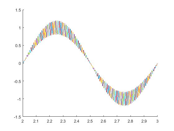
My problem is the Hermite Cubic Finite Element Space doesn't approximate $\sin(2 \pi x)$ very well using this method; the approximation wiggles a lot. Below is my plot using a Mesh with 100 elements, and using a resolution of 21.

I repeated the same procedure as above except using a Lagrange Cubic Finite Element Space, so that the shape functions over $K_R$ satisfy \begin{align*} N_1(-1) = 1, N_1(-1/3) = 0, N_1(1/3) = 0, N_1(1) = 0, \\ N_2(-1) = 0, N_2(-1/3) = 1, N_2(1/3) = 0, N_2(1) = 0, \\ N_3(-1) = 0, N_3(-1/3) = 0, N_3(1/3) = 1, N_3(1) = 0, \\ N_4(-1) = 0, N_4(-1/3) = 0, N_4(1/3) = 0, N_4(1) = 1. \end{align*}

Here is what the Lagrange shape functions look like:

With $u_1, u_2, u_3, u_4$ corresponding to $-1, -1/3, 1/3, 1$, the approximation I used on each element was $u(x) \approx u_1 N_1(x) + u_2 N_2(x) + u_3 N_3(x) + u_4 N_4(x)$. Doing this gets me much nicer results:

What is the deal? Why does the Lagrange FE space work so nice, and the Hermite FE space fail? This might be more of a "numerical analysis" question rather than a "scientific computing" question, but I thought I would try here first.

---

EDIT:

One of the comments suggested to use the formula $u(x) \approx u_1 N_1(x) + u_2 N_2(x) + u_1' N_3(x) + u_2' N_4(x)$ instead of $u(x) \approx u_1 N_1(x) + u_2 N_2(x) + u_1 N_3(x) + u_2 N_4 (x)$. I agree that using this formula is what I should have done in this first place. I implement this by computing $u_1' = 2\pi \cos(2\pi a)$ and $u_2' = 2\pi \cos(2\pi b)$ for each element $K = [a,b]$. Then my Hermite approximation to $\sin(2 \pi x)$ looks like:

Which is clearly very wrong. In case it helps, here is the MATLAB code for my problem. I use a few of my own finite element computer programs here.

% Make the mesh:
domain = [2,3]; nElement = 100;
Mesh = mesh_generator_1d(domain, nElement);

% Form a data structure to access the finite element basis:
iDegree = 3; Fem = femherm1d(Mesh, iDegree); hDegree = 1;

% Create an array with the first 100 entries corresponding to the values
% of sin(2*pi*x) evaluated at the Mesh nodes:
uGlobal = sin(2*pi*Fem.point(1:nElement+1)); iDerivative = 0;

% Extend the array so that the last 100 entries correspond to the values of
% 2*pi*cos(2*pi*x) evaluated at the Mesh nodes:
uGlobal(nElement+2:2*(nElement+1)) = 2*pi*cos(2*pi*Fem.point(nElement+2:2*(nElement+1)));

% Set the resolution and prepare the figure:
reso = 20; figure(1); clf; hold on;
uInterpolate = zeros(1,(reso+1)*size(Mesh.element,2));

for k = 1:size(Mesh.element,2) % Loop over each element in the mesh
    element = Mesh.node(Mesh.element(:,k)); % Extract element endpoints
    uLocal = uGlobal(Fem.T(:,k)); % uLocal(1) = u1, uLocal(2) = u2, uLocal(3) = u1', uLocal(4) = u2'
    x = linspace(element(1), element(2), reso+1); % x contains the points we are evaluating the shape functions at
    uInterpolate(((k-1)*(reso+1)+1):(k*(reso+1))) = evalfeherm1d(x, uLocal, ...
        element, hDegree, iDerivative); % uInterpolate = u1*N1 + u2*N2 + u1'*N3 + u2'*N4
    plot(x,uInterpolate(((k-1)*(reso+1)+1):(k*(reso+1)))); % Plot the result
end
hold off

Answer 1

Short answer

You are missing the Jacobian of the transformation for the derivatives.

Long answer

The conditions that you propose for your interpolator translate into the following system of equations

$$ \begin{bmatrix} 1 &x_1 &x_1^2 &x_1^3\\ 1 &x_2 &x_2^2 &x_2^3\\ 0 &1 &2x_1 &3x_1^2\\ 0 &1 &2x_2 &3x_2^2 \end{bmatrix} \begin{bmatrix} a_{11} &a_{12} &a_{13} &a_{14}\\ a_{21} &a_{22} &a_{23} &a_{24}\\ a_{31} &a_{32} &a_{33} &a_{34}\\ a_{41} &a_{42} &a_{43} &a_{44} \end{bmatrix} = \begin{bmatrix} 1 &0 &0 &0\\ 0 &1 &0 &0\\ 0 &0 &1 &0\\ 0 &0 &0 &1 \end{bmatrix} $$

where $x_1$ and $x_2$ are the extremes of the interval, and $a_{ij}$ are the coefficients. If you want to compute the interpolation in your reference element and then use it outside of it you need to take into account the chain rule. The formula would be then

$$f(x) \approx N_1(x) u_1 + N_2(x) u_2 + |J|(N_3(x) u'_1 + N_4(x) u'_2)\quad \forall x\in [a, b]$$

with $|J| = (b - a)/2$ the Jacobian determinant of the transformation, and, for $a=-1, b=1$,

\begin{align} N_1 (x) &= \frac{1}{4} (x - 1)^2 (2 + x)\\ N_2 (x) &= \frac{1}{4} (x + 1)^2 (2 - x)\\ N_3 (x) &= \frac{1}{4} (x - 1)^2 (x + 1)\\ N_4 (x) &= \frac{1}{4} (x + 1)^2 (x - 1)\, . \end{align}

The following code computes and plots the interpolation for your function using just 3 elements.

from __future__ import division
import numpy as np
import matplotlib.pyplot as plt

def hermite_interp(fun, grad, x0=-1, x1=1, npts=101):
    jaco = (x1 - x0)/2
    x = np.linspace(-1, 1, npts)
    f1 = fun(x0)
    f2 = fun(x1)
    g1 = grad(x0)
    g2 = grad(x1)
    N1 = 1/4*(x - 1)**2 * (2 + x)
    N2 = 1/4*(x + 1)**2 * (2 - x)
    N3 = 1/4*(x - 1)**2 * (x + 1)
    N4 = 1/4*(x + 1)**2 * (x - 1)
    interp = N1*f1 + N2*f2 + jaco*(N3*g1 + N4*g2)
    return interp


def fun(x):
    return np.sin(2*np.pi*x)


def grad(x):
    return 2*np.pi*np.cos(2*np.pi*x)


a = 2
b = 3
nels = 5
npts = 100
x = np.linspace(a, b, 100)
y = fun(x)
plt.plot(x, y, color="black")
xi = np.linspace(2, 3, num=nels, endpoint=False)
dx = xi[1] - xi[0]
for x0 in xi:
    x1 = x0 + dx
    x = np.linspace(x0, x1, npts)
    y = hermite_interp(fun, grad, x0=x0, x1=x1, npts=npts)    
    plt.plot(x, y, linestyle="dashed")
plt.show()

With the following result