Nonlinear eigenvalue problem - MATLAB code

Question

I'm trying to solve a nonlinear eigenvalue problem in MATLAB, still without success. It's a problem about graphene plasmonics.

The nonlinear eigenvalue problem is given below:

\begin{equation} \frac{\epsilon_1}{\kappa_{1||n}}E_{x||n}+\frac{\epsilon_2}{\kappa_{2||n}}E_{x||n}+ \frac{i}{\omega \epsilon_0} \sum_{p=-M}^{M}\hat{\sigma}_{n-p} E_{x||p}=0 \end{equation}

\begin{equation} \kappa_{m||n}=\sqrt{(q+nG)^2-\epsilon_m (\omega/c)^2} \end{equation}

Edit: For those ones who are familiar with Physics, in order to have a clear understanding of the problem, this is a dispersion relation about a graphene sheet between two dielectrics, supporting plasmonic modes of electromagnetic waves. The graphene sheet has a spatially-periodically modulated conductivity. So $\hat{\sigma_{j}}$ are the Fourier-series coefficients of the surface conductivity, $G=2\pi/R$ is the so-called reciprocal lattice vector, when $R$ is the spatial period, $\epsilon_0$ is the vacuum permittivity, $\epsilon_m$ is the relative permittivity of the dielectrics above and below the graphene sheet, $c$ is the speed of light in vacuum, $\omega$ is the angular frequency, $q$ is the wavenumber, $E_{x||n}$ is the $n$-th diffracted order amplitude of the $x$-component electric field (when it is expander in Fourier-Floquet series). $E_{x||n}$ is in a sense the eigenvector of the problem. Below I give a relevant paper from which I saw this relation (page 46, equation 217):

https://arxiv.org/pdf/1302.2317.pdf

The parameters $\epsilon_1$, $\epsilon_2$, $\epsilon_0$, $G$, $c$, $\hat{\sigma}_{j}$ are known. The problem stands for determining $q$ (wavenumber), $\omega$ (frequency), so as for the system of the first equation to has nontrivial solution. This should lead to a solution of the dispersion relation. This system of course is a $(2M+1) \times (2M+1)$ square system of the form $Ax=0$, where $A=A(\omega, q)$. Let's consider for simplicity that $M=1$. Then the initial equation can be written as below:

\begin{equation} \begin{bmatrix} \frac{\epsilon_1}{\kappa_{1||-1}}+ \frac{\epsilon_2}{\kappa_{2||-1}} + \frac{j}{\omega \epsilon_0} \hat{\sigma}_0 & \frac{j}{\omega \epsilon_0} \hat{\sigma}_{-1} & \frac{j}{\omega \epsilon_0} \hat{\sigma}_{-2} \\ \frac{j}{\omega \epsilon_0} \hat{\sigma}_{1} & \frac{\epsilon_1}{\kappa_{1||0}}+ \frac{\epsilon_2}{\kappa_{2||0}} + \frac{j}{\omega \epsilon_0} \hat{\sigma}_0 & \frac{j}{\omega \epsilon_0} \hat{\sigma}_{-1} \\ \frac{j}{\omega \epsilon_0} \hat{\sigma}_{2} & \frac{j}{\omega \epsilon_0} \hat{\sigma}_{1} & \frac{\epsilon_1}{\kappa_{1||1}}+ \frac{\epsilon_2}{\kappa_{2||1}} + \frac{j}{\omega \epsilon_0} \hat{\sigma}_0 \end{bmatrix} \begin{bmatrix} E_{x||-1} \\ E_{x||0} \\ E_{x||1} \end{bmatrix} = 0 \end{equation}

It is clear that $A$ depends non-linearly from $\omega$, $q$.

As far as I know, I should give a specific value to $\omega$, and then solve the equation $det(A)=0$ (numerically) to find $q$. That's how one should find the exact dispersion relation (which is a curve that matches a wavenumer $q$ to every frequency $\omega$, in a certain frequency spectrum).

I should mention that, in the paper above, it is clearly said that for sharp conductivity profiles (which is the case of my interest, for example $\sigma=\begin{cases} \sigma_1, \quad 0<x<d \\ \sigma_2, \quad d<x<R \end{cases} $), this process is poorly convergent. But I want to study how slowly does it converge. I also cannot solve the problem for a sinusodial conductivity profile either, which is the uttermost case of smooth profile, so I guess the problem is computational.

Here is my MATLAB code:

  global w % angular frequency - it is global because I pass it in the function fun
c0=299792458; %speed of light
f=linspace(25*10^12,45*10^12,1000); %frequency spectrum
guess=32*2*pi*25*10^12/c0;; % initial guess for the wavenumber
for x=1:1000 % scanning for every frequency in the spectrum
w=2*pi*f(x); 
q(x)=fsolve(@fun,guess); % find the wavenumber q via fsolve
guess=q(x); % next guess is the previous solution (wavenumber)
end
plot(q,f)

The main function (heart of the code) is below:

function F=fun(q)
global w
hbc=3.161*10^-26; % hbar*c0, SI units, [J*m]
c0=299792458; %speed of light
e0=8.854*10^-12; %vacuum permittivity [F/m]
e1=1; %dielectric permittivity, air
e2=2.1; %dielectric permittivity, spacer
elcharge=1.602*10^-19; % elementary charge, [C] 
kbol=1.38*10^-23; %Boltzmann constant, SI units [J/K]
hbar=1.054*10^-34; %reduced Planck constant, SI units, [J*s]    
h=hbar*2*pi; % Planck constant
t=0.5*10^-12; %[sec]
T=300; % Temperature [K]
mc1=0.2*elcharge; %chemical potential of 1st region, [J]
mc2=0.5*elcharge; %chemical potential of 2nd region, [J]
w1=10*10^-9; %width of 1st region, [m]
w2=60*10^-9; %width of 2nd region, [m]
R=w1+w2; %spatial period
G=2*pi/R; %reciprocal lattice wavevector
M=1; % M is the cutoff of the infinite terms of the system, -M<=n<=M
hbw=hbar*w; %hbar * w
sg1=i*((kbol*T*elcharge^2)/(pi*(w+i/t)*hbar^2))*((mc1/(kbol*T))+2*log(exp(-mc1/(kbol*T))+1))+i*(elcharge^2/(4*pi*hbar))*log((2*mc1-hbar*(w+i/t))/(2*mc1+hbar*(w+i/t))); %1st region's conductivity (Kubo formula for graphene conductivity)
sg2=i*((kbol*T*elcharge^2)/(pi*(w+i/t)*hbar^2))*((mc2/(kbol*T))+2*log(exp(-mc2/(kbol*T))+1))+i*(elcharge^2/(4*pi*hbar))*log((2*mc2-hbar*(w+i/t))/(2*mc2+hbar*(w+i/t))); %2nd region's conductivity (Kubo formula)
for n=-M:M
        k1(n+M+1)=sqrt((hbc*(q+n*G))^2-e1*hbw^2);
    k2(n+M+1)=sqrt((hbc*(q+n*G))^2-e2*hbw^2);
end
sf0=(sg1*w1/R)+(sg2*w2/R);; %zeroth Fourier component
%fill the matrix of Fourier components, sf[]
for l=-2*M:2*M
        if l~=0
                sf(l+2*M+1)=sg1*sin(l*G*w1)/(R*l*G)+j*sg1*(cos(l*G*w1)-1)/(R*l*G)-sg2*sin(l*G*w1)/(R*l*G)-j*sg2*(cos(l*G*w1)-1)/(R*l*G); 
        else
                sf(l+2*M+1)=sf0;
        end
end
%forming the main matrix of the problem, of which the determinant we want to set to zero
for n=-M:M
    v0(n+M+1)=(e1/k1(n+M+1))+(e2/k2(n+M+1))+j*sf0/(hbw*e0*c0); %diagonal elements
end
A0=diag(v0);
A=A0;
for n=1:2*M
    vu=ones(1,2*M+1-n)*j*sf((4*M+2)/2-n)/(hbw*e0*c0); %upper diagonal elements
        vd=ones(1,2*M+1-n)*j*sf((4*M+2)/2+n)/(hbw*e0*c0); %down diagonal elements
    Au=diag(vu,n);
    Ad=diag(vd,-n);
    A=A+Au+Ad;
end
F=det(A);
end

As you can see, I'm trying to solve this with fsolve. For large cutoff integer $M$, the determinant becomes extremely big (or small, if I scale properly the equations with a constant number). Anyway, the problem seems unstable. Is there a way to fix my code? Or is there a way to treat the problem in a different mathematical way? My knowledge in computational linear algebra is poor.

Thank you in advance.

Answer 1

Given a nonlinear eigenvalue problem of the form $A(\lambda)x = 0$, reducing it to a real equation $\det(A(\lambda))=0$ is known to be a poor method for just the reason you've discovered yourself. The determinant is too ill-behaved for this to work on non-trivial problems.

Even for an ordinary eigenvalue problem $Ax=\lambda x$, if you have a good approximate guess at an eigenvalue $x_0$, a typical method would be something like inverse iteration, rather than Newton's method applied to $\det(A-\lambda I)$.

There is quite some literature on this topic already, you could start by trying some of the different methods listed in [1]. In particular, they discuss different ways to treat $A(\lambda)x=0$ other than through $A$'s determinant, such as through Rayleigh quotient, and list multiple methods starting on p.10.

[1] Nonlinear Eigenvalue Problems, Heinrich Voss, Chapter 115 of the Handbook of Linear Algebra https://www.mat.tuhh.de/forschung/rep/rep164.pdf

Answer 2

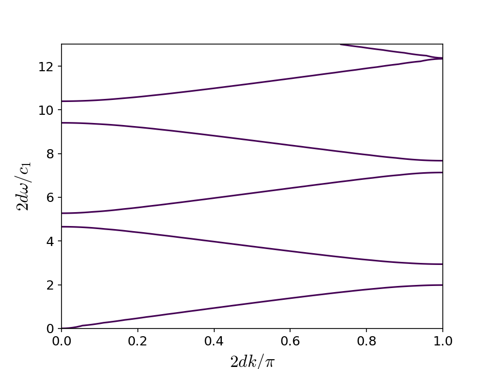
I would say that you can find the dispersion equations in the form $\omega = f(k)$ or vice-versa $k = g(\omega)$, they are not exactly equivalent. In the second form you can find complex wavenumbers. They are real for a region with propagation modes, imaginary for a region without propagation (bandgap), and they are complex for regions with attenuation.

I think that @Kirill answer is the best approach. Nevertheless, I have used another approach in the past. We can write our dispersion equation as

$$F(\omega, k) = 0\, ,$$

where we want to find all the points in a region $[0, \omega_\max] \times [0, \pi/R]$ that satisfy this relationship. If we consider a grid over this region, we can use an algorithm like marching squares for this purpose. Similar algorithms are used in contour plotting routines.

I would illustrate this approach for the dispersion relation of a bilayer material:

$$\cos(2dk) = \cos\left(\frac{\omega d}{c_1}\right)\cos\left(\frac{\omega d}{c_2}\right) - \frac{(\rho_1 c_1)^2 + (\rho_2 c_2)^2}{2\rho_1 \rho_2 c_1 c_2}\sin\left(\frac{\omega d}{c_1}\right)\sin\left(\frac{\omega d}{c_2}\right)\, ,$$

where $2d = R$, $c_i$ the speed for layer $i$, $\rho_i$ the density for layer $i$.

The following (Python) snippet does the job.

from __future__ import division, print_function
from numpy import linspace, sqrt, pi, sin, cos, meshgrid
import matplotlib.pyplot as plt

plt.rcParams["mathtext.fontset"] = "cm"
plt.rcParams["font.size"] = 12


def lhs_dispersion_bilayer(omega, d, c1, c2, rho_1, rho_2):
    factor = ((rho_1*c1)**2 + (rho_2*c2)**2)/(2*rho_1*rho_2*c1*c2)
    return cos(omega*d/c1)*cos(omega*d/c2) - factor*sin(omega*d/c1)*sin(omega*d/c2)


d = 0.5
mu_1 = 2.76e10
mu_2 = 3.47e10
rho_1 = 2770
rho_2 = 8270

c1 = sqrt(mu_1/rho_1)
c2 = sqrt(mu_2/rho_2)

omega = linspace(0, 13, 101)*c1/(2*d)
k = linspace(0, pi, 101)
k, omega = meshgrid(k, omega)
FS = cos(2*d*k) - lhs_dispersion_bilayer(omega, d, c1, c2, rho_1, rho_2)
plt.contour(k/pi, 2*d*omega/c1, FS, [0])
plt.xlabel("$2dk/\pi$", fontsize=16)
plt.ylabel("$2d\omega/c_1$", fontsize=16)
plt.ylim(0, 13)
plt.savefig("bilayer_disp.png", dpi=150)
plt.show()

And we obtain the following, that is correct.

The same approach can be done in MATLAB, or other programming languages. The solution depend on how fine is the mesh. Also, the results from this approach can be used as seeds for a Newton-Raphson iteration, if high precission is required.

Answer 3

You are trying to solve an eigenvalue problem by directly finding zeros of the determinant. This has many numerical difficulties, e.g. overflow and small convergence basin. This is the same for standard eigenvalue problems. You need techniques from numerical linear algebra. Your problem is referred to as a nonlinear eigenvalue problem which is an active field of research within numerical linear algebra.

Your problem should be reasonably easy to solve with the Julia package NEP-PACK. (I am a developer of NEP-PACK.) Your code is a bit involved so here is a simplified problem which should be easy generalize:

Similar to your post in mathexchange, you can solve $$ M(\lambda)q=0$$

where $$ M(\lambda)=A_0+A_1\lambda+A_2\sqrt{c+\lambda^2}+A_3\sqrt{d+\lambda^2} $$ as follows:

using NonlinearEigenproblems
A0=randn(10,10);
A1=randn(10,10);
A2=randn(10,10);
A3=randn(10,10); 
c=4; d=6;
f0= S->one(S)
f1= S->S
f2= S->sqrt(c*one(S)+S^2)
f3= S->sqrt(d*one(S)+S^2)
nep=SPMF_NEP([A0,A1,A2,A3],[f0,f1,f2,f3]);

and then solve it with any of the available methods, e.g., quasinewton

(omega,q)=quasinewton(nep,λ=-3.0);

it will give you a solution if the starting guess is sufficiently close to a solution since

norm((A0+A1*f1(omega)+A2*f2(omega)+A3*f3(omega))*q)

will be small. If you use this solution, please cite the package. If it leads to a publication, it would be nice to post a reference to the paper where it is used.

See a similar problem/solution in this tutorial.