Levenberg-Marquardt Algorithm for Black-box optimizations

Question

I would like to create an optimization solution for black-box software calculations. Currently, I am using the Levenberg-Marquardt algorithm to update a vector of parameters, $\beta$, with residuals, $r$, determined by outputting the black-box calculation and model parameters to a readable table.

$(J^TJ+\lambda diag(J^TJ))\delta=J^Tr(\beta)$

$\beta_{n}=\beta_{n-1} + \alpha \delta$

$r(\beta) = y_{data} - f_{model}(\beta)$

The Jacobian is estimated using Broyden's method where $\Delta f_n$ and $\Delta x_n$ are the difference in the residual vector and parameter vector between iterations respectively. Since Broyden's method is for root finding, then $\Delta f_n = r_n -r_{n-1} \rightarrow 0 $ should fit the system.

I have little experience in programming, but I think I'm close to having a solution by iterating on the following loop:

deltaf_n = np.reshape(r_n - r_old, (len(r_n), 1))  
deltabeta_n = np.reshape(beta_n - beta_old,  (len(beta_n), 1)) 
broyden_n = broyden_old + np.matmul((deltaf_n - np.matmul(broyden_old,\ 
            deltabeta_n))/np.sum(deltabeta_n**2), deltabeta_n.T)
jTj = np.matmul(broyden_n.T, broyden_n)
delta = np.linalg.solve(jTj + lam*jTj*np.eye(3), -np.matmul(broyden_n.T, r_n))
beta_old = np.copy(beta_n) 
r_old = np.copy(r_n)
broyden_old = np.copy(broyden_n)
beta_n = beta_n + alpha*delta
r_n = residuals(y_data, beta_n)

Unfortunately I'm not getting a solution because the parameters aren't updating as expected:

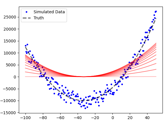
Does anyone have any idea why my parameters aren't getting updated properly? You can see that the quadratic parameter is getting updated, but for some reason the constant parameter is hardly moving.

Answer 1

The problem ended up being elsewhere in the code with complete working solution posted here:

## Python adaptation of optimization routine as conceptualized by Markus Piro circa 2014.
import matplotlib.pyplot as plt
import pandas as pd
import numpy as np
np.random.seed(42)

## function to test against
beta_true = np.array([5, 33, -1e4])
def test(x, beta):
    return beta[0]*(x+beta[1])**2 + beta[2]
## function to calculate residuals
def residuals(y_exp, beta):
    return y_exp - test(x_calc, beta)
## The true solution. The thing we are hoping to replicate through LMA
m = 50 #the number of calculated data points
x_calc = np.linspace(-100, 50, num=m)
y_true = test(x_calc, beta_true)

## synthetic experimental data. This will be used in LMA to generate fit
mult_err = np.random.uniform(low=0.8, high=1.2, size=np.shape(x_calc))
add_err = np.random.uniform(low=-1, high=1, size=np.shape(x_calc))
y_exp =  y_true * mult_err + 5e3*add_err

## Start figure where we will add traces
plot, ax1 = plt.subplots()
ax1.plot(x_calc, y_exp, 'b.', label='Simulated Data')
ax1.plot(x_calc, y_true, 'k--', label='Truth', alpha=0.6, linewidth=2.5)
ax1.set_xlim([-100,50])
ax1.set_ylim([-15000, 35000])
def trace(y_calc):
    ax1.plot(x_calc, y_calc, 'r-', alpha=0.1)

## begin process outlined in Piro et al.
## 'A Jacobian Free Deterministic Method for Solving Inverse Problems' (unpublished work)
lam = 0.1 #damping parameter
alpha = 0.2 #step length for direction vector
num_its = 100 #how many iterations to do


## initialize parameters to zero
n = np.shape(beta_true)[0] #how many parameters
beta_0 = np.reshape(np.zeros(n), (n, 1)) #initialize guess parameters to zeros
r_0 = np.reshape(residuals(y_exp, beta_0), (len(y_exp), 1)) #calculate initial residuals
beta_1 =beta_0 + 0.1*np.random.rand(n,1)#perturb initial parameter guess to produce beta_1 and calculate r_1
r_1 = np.reshape(residuals(y_exp, beta_1), (len(y_exp), 1))
r_old = np.copy(r_0)
r_k = np.copy(r_1)
beta_old = np.copy(beta_0)
beta_k = np.copy(beta_1)
broyden_old = np.zeros((m,n))
ax1.plot(x_calc, test(x_calc, beta_k), 'r-', alpha=0.3, label='Iteration')

## looping begins here
j=0
while j<=num_its:
    t_k = r_k - r_old  #calculate difference in residuals
    s_k = beta_k - beta_old #calculate difference in parameters
    y_calc = test(x_calc, beta_k) #calculate iteration trace for plotting
    trace(y_calc) #add trace to plot

    broyden_k = broyden_old + np.matmul((t_k - \
                np.matmul(broyden_old, s_k))/np.sum(s_k**2), s_k.T) #Approximate the jacobian update
    jTj = np.matmul(broyden_k.T, broyden_k) #convenience variable
    p = np.linalg.solve(jTj + lam*jTj*np.eye(n), -np.matmul(broyden_k.T, r_k)) #compute direction vector
    beta_old = np.copy(beta_k) #set up for iteration
    r_old = np.copy(r_k)
    broyden_old = np.copy(broyden_k)
    beta_k = beta_k + alpha*p
    r_k = np.reshape(residuals(y_exp, beta_k), (len(y_exp), 1))
    #print(np.sum(r_k**2), beta_k)
    j+=1

# show figure with simulated data, true solution, and iteration traces
ax1.legend()
plt.show()

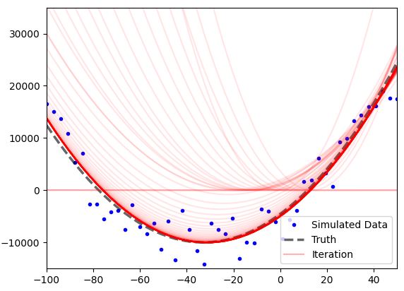
This code could be adapted to optimize a model produced in black-box software. You would need to add the capability to read tabulated data outputs and figure out some way to return the adjusted parameters back to the black-box software each iteration.