How to solve second order coupled non linear differential equations

Question

For a project I am doing, I have to solve the following system of differential equations numerically using my own code:

$$ x^2K'' = KH^2 + K(K^2-1) $$ and, $$ x^2H'' = 2K^2H + \alpha H(H^2-x^2) $$ Here, $K$ and $H$ are the dependent variables, and $\alpha$ is a parameter which I have to vary from 0 to infinity. An analytical solution exists only for $\alpha=0$ case. The boundary conditions are, $$ K(\epsilon) = 1 \\ H(\epsilon) = 0 $$ and, $$ K(\bar{\epsilon}) = 0 \\ H(\bar{\epsilon}) = \bar{\epsilon} $$ Here, $\epsilon$ is an arbitrary small number, (say 0.0001), and $\bar{\epsilon}$ is an arbitrarily large number, (say 400).

In short, boundary condition is that $K$ goes to 0 while $H$ goes to $x$.

What I have tried:

For the analytical case, I have tried RK4, RKF(Fehlberg), RK4 based Shooting, and scipy's solve_ivp. However, all suffer from the same problem, they diverge from analytical solution at around 10 (see attached graphs, first is of the two functions compared to analytical, and second is of derivatives).

I have also tried iterative finite difference approximation since I have initial guess, it suffers from same issue.

The only inbuilt function that works is solve_bvp. Can anyone suggest me two or three numerical methods for this system, for arbitrary $\alpha$, to solve as bvp and point at some good resources for those? What I have is an initial good guess for the solutions, which is the analytical solution for $\alpha=0$ case.

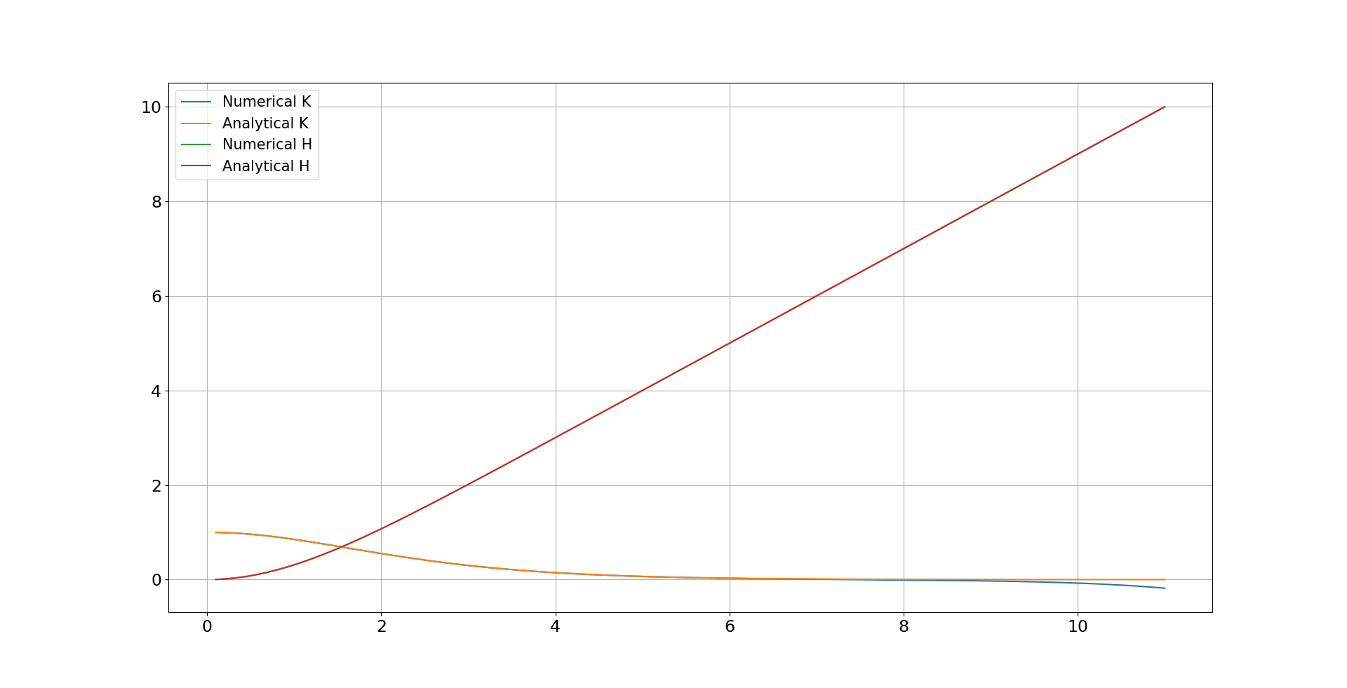
EDIT: This might be helpful. The solution for analytical case is,

$$ K = \frac{x}{\sinh(x)} $$ and $$ H = \frac{x}{\tanh(x)} - 1 $$ Edit2: Also, I even tried introducing new variables, $k$ and $h$, which: Trial1: Take out a power of x, i.e. $K=xk$ and likewise for $H$. Trial2: Take out asymptotic behavior, i.e. $K = e^{-x}k$ and $H=xh$

I recast the equations, still the same result.

UPDATE: So I tried a couple more methods and implemented solve_bvp's residual control method as well. Based on suggestion of @superbee I implemented the Finite Difference Method with Newton Ralphson technique and it works!! Briefly, I generated a system of non-linear algebraic equations by giving an initial guess and finite difference approximation. I found the Jacobian, and found an updated guess as:

$$ y^{(i+1)} = y^{(i)} - J^{-1} F $$

Answer 1

You could use a discretization method such as the finite element or finite difference method with a linearization technique such as Picard or Newton method to solve this problem. A similar question is this.

The main idea of these solution techniques is as follows:

• Pick an initial guess for the solution.
• Linearize your equation and write an updated solution in terms of a previous solution.
• Solve a sequence of linear problems until you achieve some convergence criterion.

I suggest that you check the following reference where this is explained step-by-setp.

• Hans Petter Langtangen (2013). Nonlinear differential equation problems. Available at: http://hplgit.github.io/INF5620/doc/pub/main_nonlin.pdf

Answer 2

Are you sure that you have the correct boundary conditions? I think the equation you state for the analytical case, $$H=x/\tanh(x)-1$$ is incompatible with the boundary condition $H(\bar{\epsilon})=\bar{\epsilon}$ where $\bar{\epsilon}$ is large. Maybe this is why you are getting incorrect behaviour for large $x$?

I tried solving your equation for the $\alpha=0$ case with the fixed BC $H(\bar{\epsilon})=\bar{\epsilon}-1$ and was able to find good agreement to the analytic solution using a Newton-Gauss-Seidel relaxation method.