Matlab solution for implicit finite difference heat equation with kinetic reactions

Question

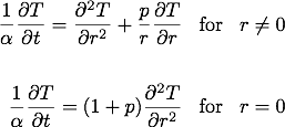
I am trying to model heat conduction within a wood cylinder using implicit finite difference methods. The general heat equation that I'm using for cylindrical and spherical shapes is:

Where p is the shape factor, p = 1 for cylinder and p = 2 for sphere. Boundary conditions include convection at the surface. For more details about the model, please see the comments in the Matlab code below.

The main m-file is:

%--- main parameters
rhow = 650;     % density of wood, kg/m^3
d = 0.02;       % wood particle diameter, m
Ti = 300;       % initial particle temp, K
Tinf = 673;     % ambient temp, K
h = 60;         % heat transfer coefficient, W/m^2*K

% A = pre-exponential factor, 1/s and E = activation energy, kJ/mol
A1 = 1.3e8;     E1 = 140;   % wood -> gas
A2 = 2e8;       E2 = 133;   % wood -> tar
A3 = 1.08e7;    E3 = 121;   % wood -> char 
R = 0.008314;   % universal gas constant, kJ/mol*K

%--- initial calculations
b = 1;          % shape factor, b = 1 cylinder, b = 2 sphere
r = d/2;        % particle radius, m

nt = 1000;      % number of time steps
tmax = 840;     % max time, s
dt = tmax/nt;   % time step spacing, delta t
t = 0:dt:tmax;  % time vector, s

m = 20;         % number of radius nodes
steps = m-1;    % number of radius steps
dr = r/steps;   % radius step spacing, delta r

%--- build initial vectors for temperature and thermal properties
i = 1:m;
T(i,1) = Ti;    % column vector of temperatures
TT(1,i) = Ti;   % row vector to store temperatures 
pw(1,i) = rhow; % initial density at each node is wood density, rhow
pg(1,i) = 0;    % initial density of gas
pt(1,i) = 0;    % inital density of tar
pc(1,i) = 0;    % initial density of char

%--- solve system of equations [A][T]=[C] where T = A\C
for i = 2:nt+1

    % kinetics at n
    [rww, rwg, rwt, rwc] = funcY(A1,E1,A2,E2,A3,E3,R,T',pw(i-1,:));
    pw(i,:) = pw(i-1,:) + rww.*dt;      % update wood density
    pg(i,:) = pg(i-1,:) + rwg.*dt;      % update gas density
    pt(i,:) = pt(i-1,:) + rwt.*dt;      % update tar density
    pc(i,:) = pc(i-1,:) + rwc.*dt;      % update char density
    Yw = pw(i,:)./(pw(i,:) + pc(i,:));  % wood fraction
    Yc = pc(i,:)./(pw(i,:) + pc(i,:));  % char fraction
    % thermal properties at n
    cpw = 1112.0 + 4.85.*(T'-273.15);   % wood heat capacity, J/(kg*K) 
    kw = 0.13 + (3e-4).*(T'-273.15);    % wood thermal conductivity, W/(m*K)
    cpc = 1003.2 + 2.09.*(T'-273.15);   % char heat capacity, J/(kg*K)
    kc = 0.08 - (1e-4).*(T'-273.15);    % char thermal conductivity, W/(m*K)
    cpbar = Yw.*cpw + Yc.*cpc;  % effective heat capacity
    kbar = Yw.*kw + Yc.*kc;     % effective thermal conductivity
    pbar = pw(i,:) + pc(i,:);   % effective density
    % temperature at n+1
    Tn = funcACbar(pbar,cpbar,kbar,h,Tinf,b,m,dr,dt,T);

    % kinetics at n+1
    [rww, rwg, rwt, rwc] = funcY(A1,E1,A2,E2,A3,E3,R,Tn',pw(i-1,:));
    pw(i,:) = pw(i-1,:) + rww.*dt;
    pg(i,:) = pg(i-1,:) + rwg.*dt;
    pt(i,:) = pt(i-1,:) + rwt.*dt;
    pc(i,:) = pc(i-1,:) + rwc.*dt;
    Yw = pw(i,:)./(pw(i,:) + pc(i,:));
    Yc = pc(i,:)./(pw(i,:) + pc(i,:));
    % thermal properties at n+1
    cpw = 1112.0 + 4.85.*(Tn'-273.15);
    kw = 0.13 + (3e-4).*(Tn'-273.15);
    cpc = 1003.2 + 2.09.*(Tn'-273.15);
    kc = 0.08 - (1e-4).*(Tn'-273.15);
    cpbar = Yw.*cpw + Yc.*cpc;
    kbar = Yw.*kw + Yc.*cpc; 
    pbar = pw(i,:) + pc(i,:);
    % revise temperature at n+1
    Tn = funcACbar(pbar,cpbar,kbar,h,Tinf,b,m,dr,dt,T);

    % store temperature at n+1
    T = Tn;
    TT(i,:) = T';
end

%--- plot data
figure(1)
plot(t./60,TT(:,1),'-b',t./60,TT(:,m),'-r')
hold on
plot([0 tmax/60],[Tinf Tinf],':k')
hold off
xlabel('Time (min)'); ylabel('Temperature (K)');
sh = num2str(h);  snt = num2str(nt);  sm = num2str(m);
title(['Cylinder Model, d = 20mm, h = ',sh,', nt = ',snt,', m = ',sm])
legend('Tcenter','Tsurface',['T\infty = ',num2str(Tinf),'K'],'location','southeast')

figure(2)
plot(t./60,pw(:,1),'--',t./60,pw(:,m),'-','color',[0 0.7 0])
hold on
plot(t./60,pg(:,1),'--b',t./60,pg(:,m),'b')
hold on
plot(t./60,pt(:,1),'--k',t./60,pt(:,m),'k')
hold on
plot(t./60,pc(:,1),'--r',t./60,pc(:,m),'r')
hold off
xlabel('Time (min)'); ylabel('Density (kg/m^3)');

The function m-file, funcACbar, that creates the system of equations to solve is:

% Finite difference equations for cylinder and sphere
% for 1D transient heat conduction with convection at surface
% general equation is:
% 1/alpha*dT/dt = d^2T/dr^2 + p/r*dT/dr for r ~= 0
% 1/alpha*dT/dt = (1 + p)*d^2T/dr^2     for r = 0
% where p is shape factor, p = 1 for cylinder, p = 2 for sphere

function T = funcACbar(pbar,cpbar,kbar,h,Tinf,b,m,dr,dt,T)

alpha = kbar./(pbar.*cpbar);    % effective thermal diffusivity
Fo = alpha.*dt./(dr^2);         % effective Fourier number
Bi = h.*dr./kbar;               % effective Biot number

% [A] is coefficient matrix at time level n+1
% {C} is column vector at time level n
A(1,1) = 1 + 2*(1+b)*Fo(1);
A(1,2) = -2*(1+b)*Fo(2);
C(1,1) = T(1);

for k = 2:m-1
    A(k,k-1) = -Fo(k-1)*(1 - b/(2*(k-1)));   % Tm-1
    A(k,k) = 1 + 2*Fo(k);                    % Tm
    A(k,k+1) = -Fo(k+1)*(1 + b/(2*(k-1)));   % Tm+1
    C(k,1) = T(k);
end

A(m,m-1) = -2*Fo(m-1);
A(m,m) = 1 + 2*Fo(m)*(1 + Bi(m) + (b/(2*m))*Bi(m));
C(m,1) = T(m) + 2*Fo(m)*Bi(m)*(1 + b/(2*m))*Tinf;

% solve system of equations [A]{T} = {C} where temperature T = [A]\{C}
T = A\C;

end

And finally the function that deals with the kinetic reactions, funcY, is:

% Kinetic equations for reactions of wood, first-order, Arrhenious type equations
% K = A*exp(-E/RT) where A = pre-exponential factor, 1/s
% and E = activation energy, kJ/mol

function [rww, rwg, rwt, rwc] = funcY(A1,E1,A2,E2,A3,E3,R,T,pww)

K1 = A1.*exp(-E1./(R.*T));    % wood -> gas (1/s)
K2 = A2.*exp(-E2./(R.*T));    % wood -> tar (1/s)
K3 = A3.*exp(-E3./(R.*T));    % wood -> char (1/s)

rww = -(K1+K2+K3).*pww;      % rate of wood consumption (rho/s)
rwg = K1.*pww;               % rate of gas production from wood (rho/s)
rwt = K2.*pww;               % rate of tar production from wood (rho/s)
rwc = K3.*pww;               % rate of char production from wood (rho/s)

end

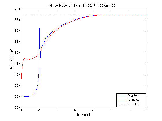
Running the above code gives a temperature profile at the center and surface of the wood cylinder:

As you can see from this plot, for some reason the center and surface temperatures rapidly converge at the 2 min mark which isn't correct.

Any suggestions on how to fix this or create a more efficient way to solve the problem?

Answer 1

It looks like the model you're trying to solve is:

\begin{align} (1/\alpha(w,c))T_{t}(r,t) &= T_{rr}(r,t) + (p/r) \cdot T_{r}(r,t) \\ w_{t}(r,t) &= -(k_{1}(T(r,t)) + k_{2}(T(r,t)) + k_{3}(T(r,t)))w(r,t) \\ g_{t}(r,t) &= k_{1}(T(r,t))w(r,t) \\ a_{t}(r,t) &= k_{2}(T(r,t))w(r,t) \\ c_{t}(r,t) &= k_{3}(T(r,t))w(r,t) \end{align}

where:

• $r =$ radius
• $t =$ time
• $T =$ temperature
• $w =$ wood density
• $g =$ gas density
• $a =$ tar density
• $c =$ char density
• $k_{i}$ is a rate coefficient for $i = 1, 2, 3$
• $\alpha$ is a thermal diffusivity that is a function of $w$ and $c$
• $p$ is a constant shape factor

and subscripts of $t$ and $r$ denote derivatives.

You only have boundary conditions for temperature (which are the only boundary conditions you need). Although you mention the convection boundary condition at the surface, your other boundary condition should be a symmetry condition: $T_{r}(r = 0, t) = 0$ for all time, which you should impose as part of the system you form in funcACbar, rather than omitting that term from the PDE at $r=0$ and discretizing the resulting equation.

It seems like you're using some sort of two-stage implicit predictor-corrector-like scheme to integrate the equations for temperature, where you do the following:

\begin{align} \tilde{T}(r, t_{n+1}) &= T(r, t_{n}) + hf(\tilde{T}(r, t_{n + 1})) \\ T(r, t_{n + 1}) &= \tilde{T}(r, t_{n + 1}) + hf(T(r, t_{n + 1})) \end{align}

where the function $f$ denotes the right-hand side of the differential equation for $T$ (it's really a function of more variables, but you treat the other variables as essentially constant over each of the two stages of your integrator.

Within each stage, you advance the species densities using explicit Euler.

I see a couple potential problems with this scheme:

• Since temperature is really coupled to the wood and char densities, you're introducing what is called a (physics) splitting error that could be causing the numerical artifacts you've mentioned. Shrinking your time step will reduce this error.
• Chemical source terms are sometimes stiff. You're integrating them with explicit Euler, which I wouldn't think to do intuitively (based on the problems I study), due to stability issues. However, for most of your problem, there doesn't seem to be any great instability, and any instabilities you have are damped out, so maybe that's not an issue. Combining explicit and implicit methods in this way usually limits accuracy to first or second-order (depending on splitting), unless you use IMEX (implicit-explicit) methods.
• Your biggest problem is rolling your own time integrator, so you have no accuracy control. Or rather, your only way to control accuracy is to shrink the time step, look at your solution, and see if the new solution is more accurate.

Here's what I would do:

• Discretize your equations in space, and solve all of them simultaneously (for now). If you have twenty points in the radial direction, and five state variables in the continuous formulation of your PDE, you'll only have 100 state variables in your right-hand side. MATLAB should be able to handle that fairly easily. Implementing this suggestion will eliminate splitting errors.
• For time integration, use something from a library. Given that you have diffusion terms and chemistry terms, you probably want to use something implicit. If you find that none of the built-in MATLAB integrators work, download the MATLAB interface to SUNDIALS, install it, and use CVODE. Implementing this suggestion will give you error-controlled time integration, and these integrators will adapt their time steps to satisfy error tolerances you supply, so you can ask for solutions that are more accurate or less accurate depending on your accuracy requirements.

After you do those things, it will be easier to troubleshoot your problems.