Failing integration with the radau5-implementation in DotNumerics, over a discontinuity

Question

Summary

We are trying to solve some models of emission of substances to the air. In these models, emission stops at a certain point.

We are using the DotNumerics implementation of radau5

We had issue finding correct solutions. If emission stops, the air concentration should drop, but this was not always the case.

We were able to reproduce this issue with a simple model for which we could also find the analytic solution. Also, we inspected the radau5 source code and found a test that looks like an optimization. Due to this test many evaluations of the Jacobian are skipped. If we remove this test, the results are a lot better.

We have also used the implicit fourth order Runge Kutta by Press et all., Numerical Recipes 2nd edition for our original problems and this method did not show this issue. We didn't find the time to test it on this problem.

We wonder:

1. What is this test? Is there some documentation on it?
2. Can we safely remove the test to skip evaluation of the Jacobian?
3. Can we expect radau5 to cope with discontinuities, or should we integrate the two trajectories separately?

Detailed information

The model consists of two compartments. Initially, compartment I contains the substance that is emitted to compartment II. From compartment II, product is removed by ventilation.

$$ \begin{array}{rclr} \frac{dC_I}{dt}&=&-k_{12}(C_I- C_{II}) \\ \frac{dC_{II}}{dt}&=&k_{12}(C_I- C_{II})-k_{02}C_{II} & t < T \\ \frac{dC_{II}}{dt}&=&-k_{02}C_{II} & t > T \\ C_I (0)&=&1 \\ C_{II}(0)&=&0 \end{array} $$

We found these analytic solutions:

$$ \begin{array}{rclr} C_{II}(t)&=&C_{II}(T)e^{-k_{02}(t-T)} \\ &=&\frac{C_0}{\sqrt{D}}k_{12}(e^{λ_+ T}-e^{λ_-T})e^{-k_{02}(t-T)} & t < T \\ C_{II}(t)&=&\frac{C_0}{\sqrt{D}} k_{12} (e^{λ_+t}-e^{λ_- t}) & t > T \\ D&=&4k_{12}^2+k_{02}^2 \\ λ_±&=&-k_{12}-\frac{k_{02}}{2}±\frac{\sqrt{D}}{2} \end{array} $$

We implemented this model in C#.

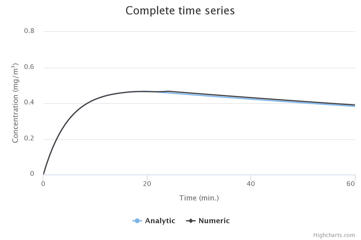
The numeric solution with a tolerance of 0.01 is as follows:

jsfiddle for original radau5 and relative tolerance: 0.01

In this case, the Jacobian is evaluated only twice.

Looking through the radau5 code, we found a test:

if (THETA <= THET) goto LABEL20;

on line 1663 in .\DotNumerics\ODE\Radau5\radau5.cs,

IF (THETA.LE.THET) GOTO 20

on line 1073 in http://www.unige.ch/~hairer/prog/stiff/radau5.f.

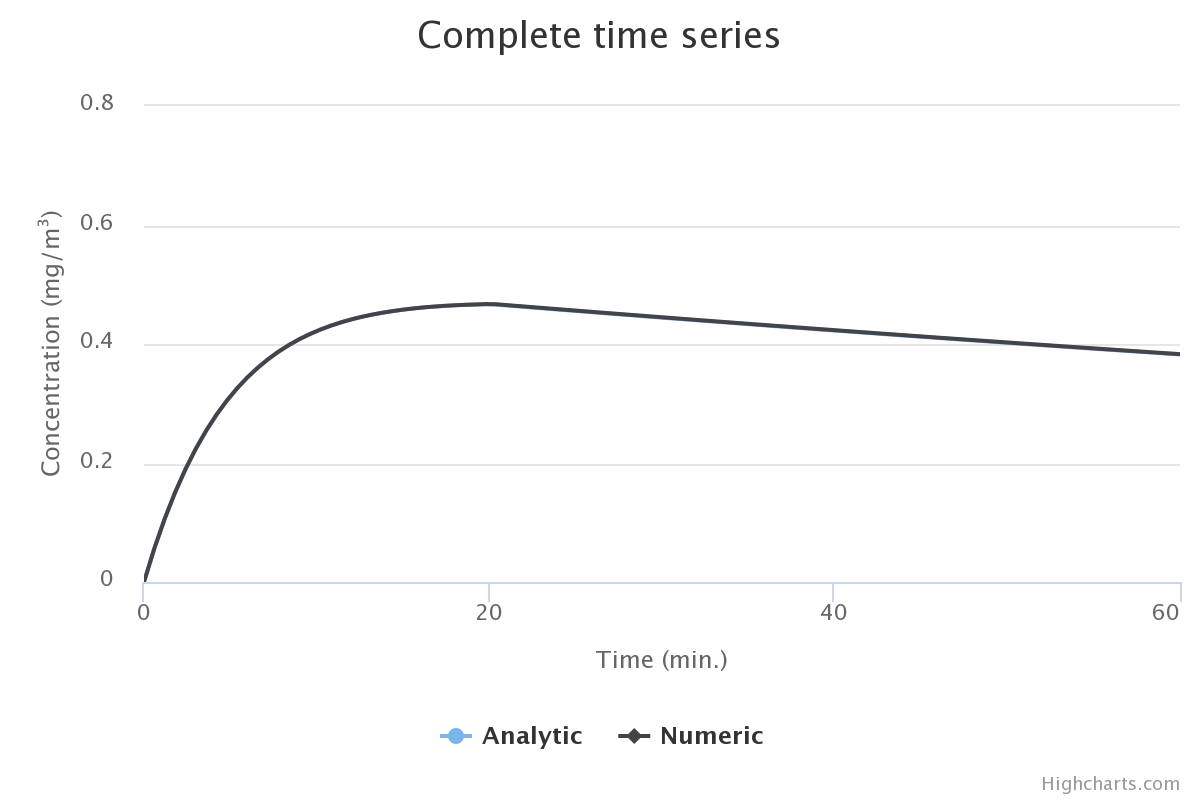
If we apply the fix we get:

jsfiddle for original radau5 and relative tolerance: 0.01

Reducing the tolerance to 0.001 yields better result, with or without fix.

jsfiddle for original radau5 and relative tolerance: 0.001 jsfiddle for modified radau5 and relative tolerance: 0.001

However, without fix, the Jacobian is still evaluated only three times, so that could be a coincidence.

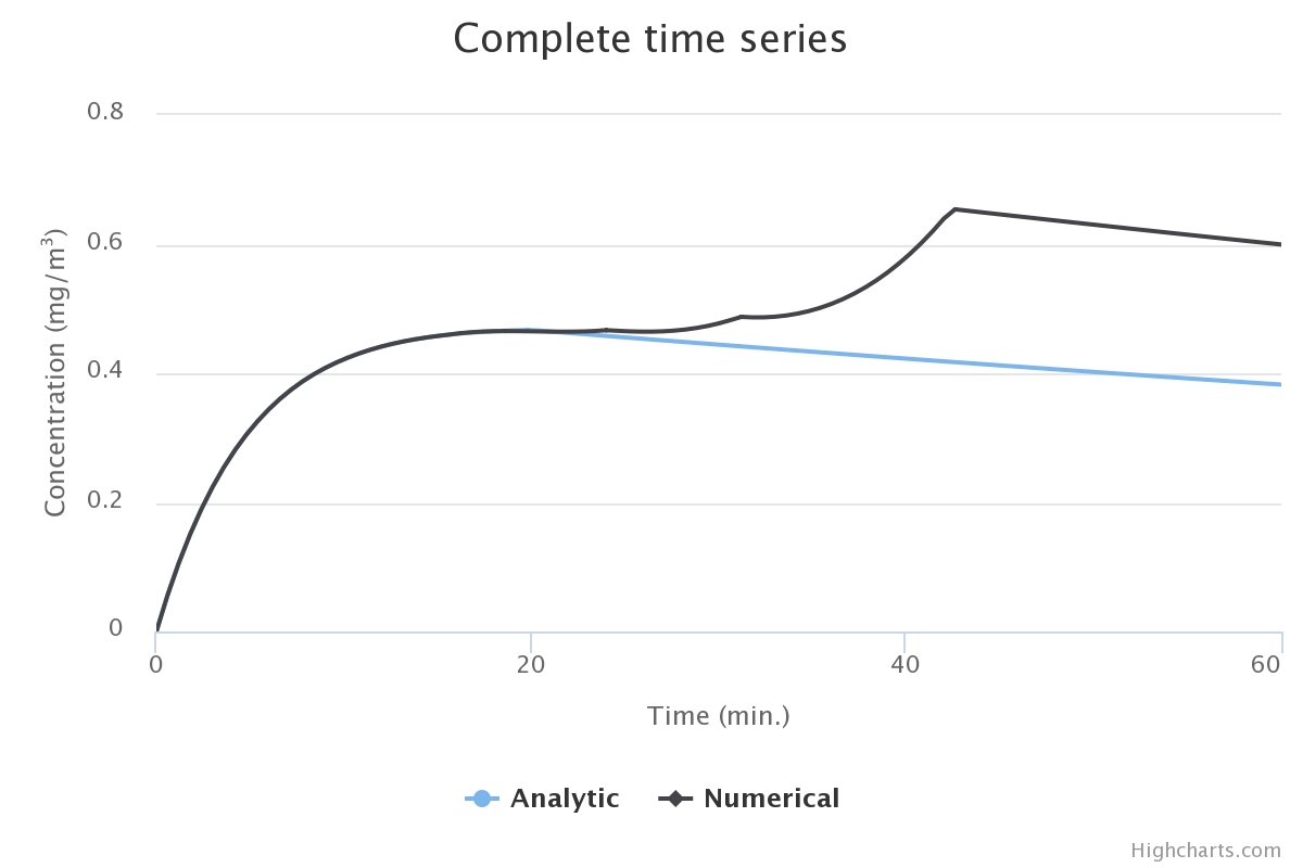
A c# solution that demonstrates this is on GitHub.

Answer 1

First of all, I cannot judge the quality of the DotNumerics implementation of Radau5, I can only assume it is a direct port of the Fortran original from Hairer and Wanner. A full description of their Radau5 implementation is in their book on solving stiff differential equations.

The test you refer to is a check to see if the Jacobian should be recomputed. If you don't provide an explicit Jacobian, Radau will try to estimate this Jacobian by finite differences. The Radau code computes, based on the Newton iterations a parameter "theta". If this value is larger than a certain threshold ("THET"), the Jacobian is recomputed. The user has the option to set the value of THET (at least in the Fortran implementation) by means of the WORK(3) variable. So don't change anything in the code! Use this option to find good values for THET. According to the Fortran implementation, the default for WORK(3) is 0.001. You could check if in the DotNumerics implementation this default value is kept. Again, in the FORTRAN implementation, setting WORK(3) to a negative value will skip the test and re-evaluate the Jacobian at every time step (probably more accurate, but also more expensive).

Second, I ran your problem as you describe using Assimulo in Python. See the code below. The solution gets rougher, but I don't observe the jump

Third, if I understand it correctly, you know your "cross-over" point $T$ explicitly, i.e. it is not problem/simulation dependent. So why make life hard on Radau by having a discontinuity in the right-hand-side of the ODE? Why not simply integrate up to $t = T$ and then use those values as initial values for the next problem?

Finally, if further on you wish to have "problem-dependent" discontinuities, I suggest to use the CVODE code which implements a very nice way to handle state changes. See for example my answer to a recent question on how to stop a simulation if a certain condition has been met and the example on the Assimulo website describing a pendulum problem where the pendulum hits a wall.

Code example

import numpy as np
from assimulo.problem import Explicit_Problem
from assimulo.solvers import Radau5ODE
import matplotlib.pyplot as plt
%matplotlib inline

C0 = 1.0
T = 20.0
tf = 60.0
k02 = 0.005
k12 = 0.1

def rhs(t,y):

    ydot = np.zeros_like(y)

    if t <= T:
        ydot[0] = k12 * (y[1] - y[0]) - k02 * y[0]
        ydot[1] = -k12 * (y[1] - y[0])
    else:
        ydot[0] = -k02 * y[0]
        ydot[1] = 0.0

    return ydot

y0 = np.array([C0,0.0])

model = Explicit_Problem(rhs,y0)
simulation = Radau5ODE(model)
simulation.rtol = 1e-2

t, y = simulation.simulate(60.)
simulation.reset()

Running this gives the following output

    Final Run Statistics: --- 

 Number of steps                                 : 9
 Number of function evaluations                  : 48
 Number of Jacobian evaluations                  : 2
 Number of function eval. due to Jacobian eval.  : 4
 Number of error test failures                   : 0
 Number of LU decompositions                     : 9

Solver options:

 Solver                  : Radau5 (explicit)
 Tolerances (absolute)   : 0.01
 Tolerances (relative)   : 0.01

Simulation interval    : 0.0 - 60.0 seconds.
Elapsed simulation time: 0.0007725144052983524 seconds.

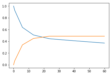
and plotting both concentrations gives

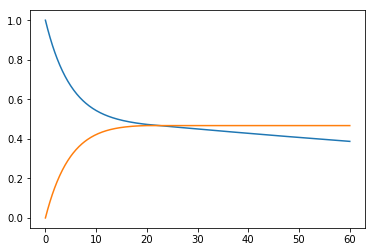
For completeness, this is the plot for a requested absolute and relative tolerance of 1e-12.

Which is different from what you observe: in this simulation there is no decrease (I took the values for the coefficients from your Github code).

Answer 2

Can we expect radau5 to cope with discontinuities, or should we integrate the two trajectories separately?

Differential equation methods cannot easily handle discontinuities like this. If you step over a discontinuity, you cannot prove that you will not have order loss. In fact, you normally will have loss of accuracy. Because of this, you want to make sure you hit each discontinuity "exactly", i.e. step right on it (or integrate the two pieces separately).

A case study for this is delay differential equation solvers where an initial discontinuity gets propagated, and the goal of a delay equation solver is to use an ODE method with an interpolation in a specific way that you track and hit the discontinuities. From this it's very well quantified how error-costly it is to not track discontinuities.