I am by no means experienced with the wave equation, but I think the issue comes from the imposition of the periodic BCs.
The periodic boundary conditions can be imposed by using ghost points: you do as if you were considering an extended system which, in Python terms, would have the state vector:
u_extend=[u[-1], u[0], u[1], ..., u[M-1], u[M], u[0]]
The bold values are duplicated values from the outer points of the original values. They allow to apply the laplacian operator easily at the boundaries.
Remark: For a Neumann BC $\partial_x u(x=0,t)=\partial_x u(x=L,t) = 0$, the ghost points would instead be (at first-order):
u_extend=[u[0], u[0], u[1], ..., u[M-1], u[M], u[M]]
This is actually the reason why your code does have M+2 space points, and not just M. Points 1 and M+2 (so 0 and M+1 in Python indices) are meant to be your ghost points. However you were not handling them correctly, you were only setting the value of the ghost point at point M+2, not the ghost point at point 0. Also I am quite confused with your usage of new_u which I think is not correct, as you basically replace your whole solution history with zeros, apart from the last step...
Here is a revision of your code, with comments to describe my corrections:
import numpy as np
import matplotlib.pyplot as plt


class wave_eq:
    def __init__(self,init_m,init_n):
        self.M = init_m
        self.N = init_n

        # self.x_grid = np.linspace(0, 1,self.M + 2) # no need for [ ... ]
        # I think this space grid introduces a small error in the placement of
        # the outer nodes with respect to the imposition of the boundary condition
        # better to use:
        self.x_grid = np.linspace(0,1,self.M)
        # AND then add the ghost point location
        dx = self.x_grid[1]-self.x_grid[0]
        self.x_grid = np.hstack((-dx, self.x_grid, self.x_grid[-1]+dx ))
        # then your "true" points really go from x=0 to x=1

        self.t_grid = np.linspace(0, 1, self.N + 2)
        self.solution = []


    def forward_euler_solver(self,g):
        M = self.M
        N = self.N

        h = self.x_grid[1] - self.x_grid[0]
        k = self.t_grid[1] - self.t_grid[0]

        r = k/h
        u = np.zeros(shape = (M+2,N+2)) # initial time + (N+1) forward steps

        u[:,0] = g(self.x_grid) #apply initial condition u(x,0) = g(x)

        print(N,M,len(self.t_grid))
        for i in range(N+1):
            print('time step {}/{}'.format(i+1,N+1))
            # for j in range(M+1): # better if vectorised
            if (i == 0): #using Neumann condition at first time step
                # new_u[j][i] = u[j][i]   + ((r**2)/2)*(u[j+1][i] - 2*u[j][i]   + u[j-1][I])
                u[1:-1,i+1]   = u[1:-1,i] +  (r**2)   *(u[2:,i]   - 2*u[1:-1,i] + u[:-2,i])
                # --> r**2, not (r*2)/2
                # --> i, not I
            else:
                # new_u[j][i] = 2*u[j][i]   - u[j][i-1]   + (r**2)*(u[j+1][i] - 2*u[j][i]   + u[j-1][i])
                u[1:-1,i+1]   = 2*u[1:-1,i] - u[1:-1,i-1] + (r**2)*(u[2:,i]   - 2*u[1:-1,i] + u[:-2,i])

            #new_u[-1][i] = new_u[0][i] #Apply periodic boundary condition
            #Apply periodic boundary condition by using the ghost points
            u[ 0,i+1]  = u[-3,i+1] # on the left side
            u[-1,i+1]  = u[ 2,i+1]  # on the right side

            # u[ 0,i+1]  = u[-2,i+1] would be incorrect !
            # u[ 0,i+1]  = u[ 1,i+1] would be incorrect !

        self.solution = u


def init_c_g(x):
    return np.cos(4*np.pi*x)


def analytical_sol(t,x):
    # only for c=1
    return 0.5 *( np.cos(4*np.pi*(x-t)) + np.cos(4*np.pi*(x+t)) )

obj = wave_eq(init_m=100, init_n=1000)
obj.forward_euler_solver(g=init_c_g)

#%%
nt = obj.solution.shape[1]
ylim = [np.min(obj.solution), np.max(obj.solution)]

for i in range(1,nt,200): # plot every several time step
    plt.figure()
    plt.plot(obj.x_grid, obj.solution[:,i])
    plt.plot(obj.x_grid, analytical_sol(obj.t_grid[i], obj.x_grid))
    plt.ylim(ylim)
    plt.grid()
    plt.xlabel(r'$x$')
    plt.ylabel(r'$u$')
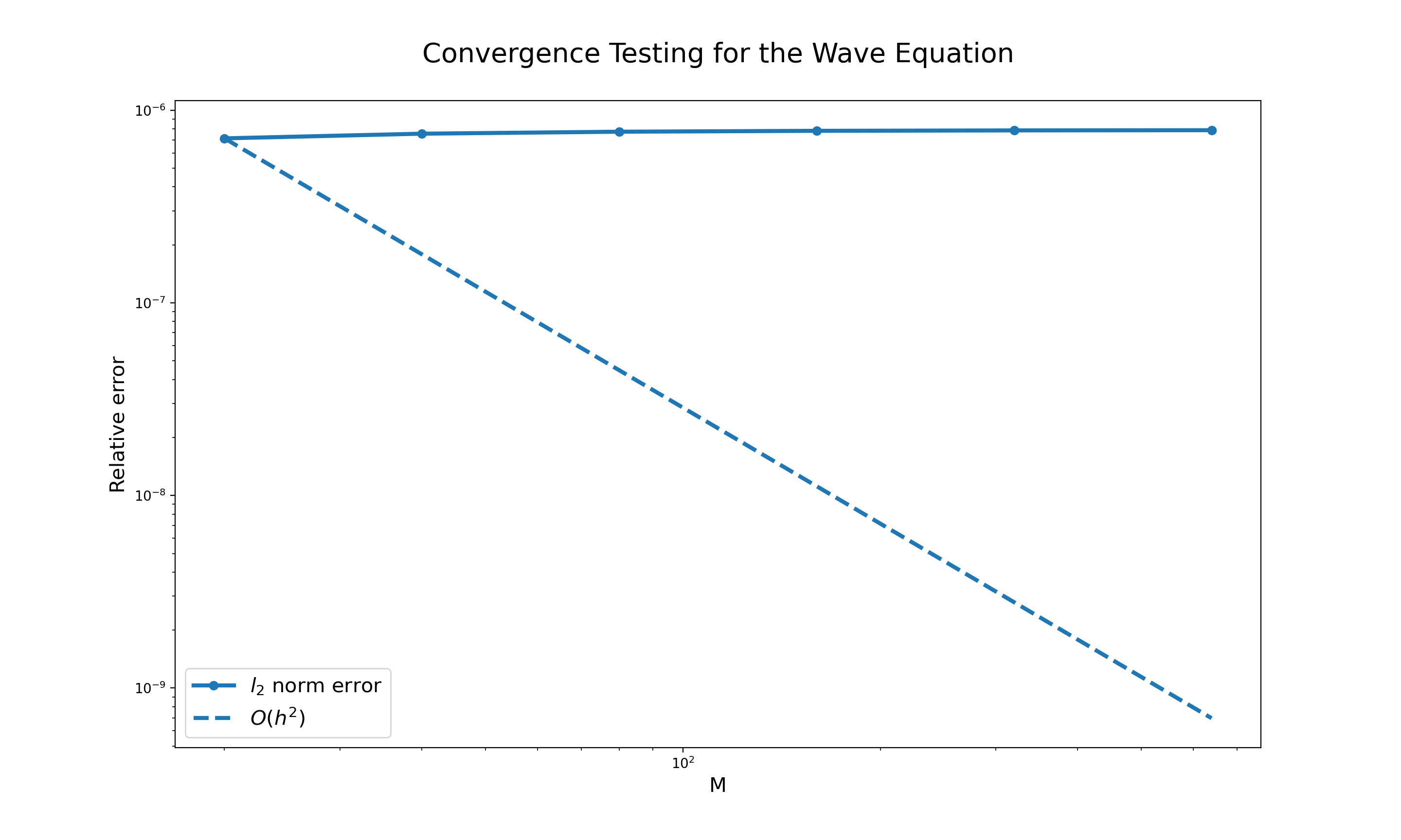
Also on a side note, for you convergence analysis, I assume you have a fixed time step value that does not change when the number of mesh points is increased. That may cause the error of the time discretisation to dominate the overall error for highly refined grids. Just in case, the convergence analysis is performed in the last part of the code snippet.
How to improve the error
There are two sources of error: the space discretisation (the discrete laplacian you use is second-order accurate), and the temporal scheme (here only first-order accurate). So your error (at one point in space) is $\epsilon= O(\Delta t) + O(\Delta x^2) = O(1/N) + O(1/M^2)$.
You can improve the error at least in two ways:
- take smaller space and time steps
- use higher-order schemes, both in space and time.
My initial answer with adaptive time stepping ensures that the error coming from the time discretisation is both high-order and very low, thus you get $\epsilon \approx O(\Delta x^2)$, i.e. you only see the error of your spatial scheme. You could try using high-order finite differences (see https://en.wikipedia.org/wiki/Finite_difference_coefficient#Central_finite_difference for coefficients), however they will require adding additional ghost points, because the spatial scheme's stencil will extend.
I've complemented my own code with a generic laplacian soatial scheme with orders 2, 4 or 6 (coefficients taken from the previous wiki page). They work very well, and actually led me to realise that there is another issue with the ghost points used here: points 0 and points N are actually duplicates, i.e. they are supposed to be identical at all times if periodic conditions are used. Therefore, the left ghost point should not be u[-1] but u[-2] for example. Doing so has greatly improved the convergence, as well as made the adaptive integration much quicker, as the laplacian was previously not smooth at the boundaries. Otherwise you could just drop your last mesh point.
The following figure shows your mesh (in thick blue), and the "ghost" meshes used for the periodicity. It is clear that u[0]=u[-1] at all times, and that the correct ghost points are u[-2] (left) and u[1] (right).

Appendix
Here is my first answer for completeness, with a code I wrote to solve this problem. I reformulated the 2nd-order system ODE as a system of 1st-order ODE by introducing $v = \partial_t u$ as additional field. I use a standard high-order adaptive ODE solver (from Scipy) to solve the semi-discrete system (after discretisation in space), so that the error from the time discretisation is negligible.
"""
The ODE d_{tt} u = c^2 d_{xx} u is trasnformed to a first-order ODE by introducing
v = du/dt:
            d/dt (u, v) = (v, c^2 d_{xx} u)
"""
import matplotlib.pyplot as plt
import numpy as np
import scipy.integrate

#%% define the problem
N = 1000 # number of mesh points
mesh = np.linspace(0,1,N) # spatial mesh
dx = mesh[1]-mesh[0] # spatial step size
c = 1. # wave speed
tf = 1. # final time
order=6 # order of the spatial scheme

# initial condition
u0 = np.cos(4*np.pi*mesh)
du0dt = 0.*u0 # initially at rest
y0 = np.vstack((u0,du0dt)).reshape((-1,), order='F') # initial solution for the first order ODE system

#%% Solve as a 1st-order ODE
coeffs = ((1,-2,1),
          (-1/12,4/3,-5/2,4/3,-1/12),
          (1/90,-3/20,3/2,-49/18,3/2,-3/20,1/90))
orders = (2,4,6)

def computeLaplacian(u,order):
    """ Finite-difference Laplacian with periodic BCs"""
    iord = orders.index(order)
    coef = coeffs[iord]
    stencil_halfwidth = int((len(coef)-1)/2) # number of required neighbours to one side
    N = u.size

    # create state vector with ghost points (ghosts_left, u, ghost_right)
    u_extended = np.zeros((N+2*stencil_halfwidth,))
    u_extended[stencil_halfwidth:-stencil_halfwidth] = u[:]
    # u_extended[0:stencil_halfwidth]  = u[-stencil_halfwidth:]
    # u_extended[N+stencil_halfwidth:] = u[:stencil_halfwidth]
    # In fact, I had to correct this, because the endpoints are actually physical duplicates...
    u_extended[0:stencil_halfwidth]  = u[-stencil_halfwidth-1:-1]
    u_extended[N+stencil_halfwidth:] = u[1:stencil_halfwidth+1]

    # compute laplacian
    laplacian = np.zeros_like(u)
    for i in range(len(coef)):
        laplacian[:] = laplacian[:] + coef[i]*u_extended[i:N+i]
    return laplacian

def laplacienOrder2(u):
    """ The original spatial scheme """
    laplacian = np.zeros_like(u)
    laplacian[1:-1] = (u[:-2] - 2*u[1:-1] + u[2:])
    #  - periodic BCs
    u_ghost_left  = u[-1]
    u_ghost_right = u[0]
    laplacian[0] = (u_ghost_left - 2*u[0] + u[1])
    laplacian[-1] = (u_ghost_right - 2*u[-1] + u[-2])
    return laplacian

def odefun(t,x, c, dx, order):
    """ first-order ODE for the wave equation c d_{tt} u = c^2 d_{xx} u """
    u, dudt = x[::2], x[1::2]
    laplacian = computeLaplacian(u,order)
    ddudtt = ((c/dx)**2)*laplacian
    return np.vstack((dudt,ddudtt)).reshape((-1,), order='F')

def analytical_sol(t,x):
    return 0.5 *( np.cos(4*np.pi*(x-t)) + np.cos(4*np.pi*(x+t)) )

#%% observe the evolution of the solution
sol = scipy.integrate.solve_ivp(fun=odefun, t_span=(0,tf), t_eval=np.linspace(0,tf,30),
                                y0=y0, method='DOP853', rtol=1e-10, atol=1e-10,
                                args=(c,dx,order))
nt = sol.t.size
u, v = sol.y[::2,:], sol.y[1::2,:]
for i in range(nt): #0,nt,max([1,int(nt/20)]) ):
    plt.figure()
    plt.plot(mesh, u[:,i], label='numerical')
    plt.plot(mesh, analytical_sol(sol.t[i], mesh), linestyle='--', label='analytical')
    plt.ylim(np.min(u),np.max(u))
    plt.grid()
    plt.legend(loc='upper right', framealpha=0)
    plt.xlabel(r'$x$')
    plt.ylabel(r'$u$')
    plt.title('t={:.2f}'.format(sol.t[i]))

#%% Convergence analysis
tf = 0.5
Nvec = np.unique(np.logspace(1,np.log10(2000),10).astype(int))
meshes, sols = [], []
for i,N in enumerate(Nvec):
    print('{}/{} (N={})'.format(i+1,len(Nvec),N))
    mesh = np.linspace(0,1,N) # spatial mesh
    dx = mesh[1]-mesh[0] # spatial step size

    # initial condition
    u0 = np.cos(4*np.pi*mesh)
    du0dt = 0.*u0 # initially at rest
    y0 = np.vstack((u0,du0dt)).reshape((-1,), order='F') # initial solution for the first order ODE system

    if 1: # adaptive solving with tight tolerances
        sol = scipy.integrate.solve_ivp(fun=odefun, t_span=(0,tf), t_eval=np.linspace(0,tf,2),
                                    y0=y0, method='DOP853', rtol=1e-13, atol=1e-13,
                                    args=(c,dx,order))
    else: #hack to get constant time steps with solve_ivp (only for explicit schemes)
        dt = 1e-3
        sol = scipy.integrate.solve_ivp(fun=odefun, t_span=(0,tf), t_eval=np.linspace(0,tf,2),
                                  y0=y0, method='DOP853', rtol=1e99, atol=1e99,
                                  max_step=dt, first_step=dt, args=(c,dx,order))
    sols.append( sol )
    meshes.append(mesh)


#%% Error analysis
error_analytical = np.zeros(( Nvec.size )) # error relative to analytical solution
error_analytical_point = np.zeros(( Nvec.size )) # error relative to analytical solution
error_finest_point = np.zeros(( Nvec.size )) # error relative to the finest numerical solution
for i in range(len(Nvec)):
    error_analytical[i] = np.sqrt( np.sum( (sols[i].y[::2,-1] - analytical_sol(tf, meshes[i]))**2 )/ meshes[i].size )
    error_analytical_point[i] = np.abs(sols[i].y[0,-1] - analytical_sol(tf, 0.))
    error_finest_point[i] = np.abs(sols[i].y[0,-1] - sols[-1].y[0,-1])

plt.figure()
dx = (1/Nvec)
plt.loglog(dx, error_analytical, marker='o', label='vs analytical (2-norm)')
plt.loglog(dx, error_analytical_point, marker='o', label='vs analytical (BC point)')
plt.loglog(dx[:-1], error_finest_point[:-1], marker='o', label='vs finest (BC point)')
iref = 0 #int(len(Nvec)/2) # used to plot reference convergence orders
plt.loglog(dx, error_analytical[iref]*(dx/dx[iref])**(order), label='order {}'.format(order), linestyle='--', color='r')
plt.loglog(dx, error_analytical[iref]*(dx/dx[iref])**(2*order), label='order {}'.format(2*order), linestyle='--', color='b')
plt.legend()
plt.grid()
plt.xlabel('dx')
plt.ylabel('error')
plt.ylim(1e-16, 1e-2)
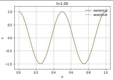
Here are the numerical and analytical solutions after 1 seconds (1000 mesh points):
And here is the convergence result for the 6-th order scheme:
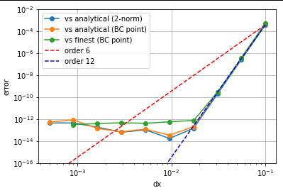
Here, the 6-th order spatial scheme converges with order 12, and (4th-order reaches order 8, 2nd-order reaches order 4...) I am not sure if I missed something, but that is strange !
As I said, I am not experienced with this kind of problem, so I am open to remarks and suggestions !


dudxx[0] = (u[1] - 2*u[0] + u[-1])/dx**2. Do a similar thing on the opposite side and that should work. $\endgroup$