Why is this scipy.root code not converging?

Question

I'm running a test problem to set up larger problems. Solving the simple unsteady heat equation via finite differences:

$$ \frac{\partial T}{\partial t} = \alpha \frac{\partial^2T}{\partial x^2}$$

$\alpha = 0.001$

$T(x=0,t) = 60°C$

$T(x=L,t) = 25°C$

$T(x,t=0) = 25°C$

import matplotlib.pyplot as plt
import numpy as np
import sympy as sp
from scipy.optimize import fsolve
from scipy import optimize
import pandas as pd
from numba import njit

t_max = 25
x_max = 1
N_points_1 = 61
N_points_2 = 11
dt = t_max/(N_points_1-1) 
dx = x_max/(N_points_2-1)
N_variables = N_points_1 * N_points_2
alpha = 0.01 
T_x_0 = 60 
T_x_L = 25
T_t_0 = 25

@njit
def EDP (v):
    T_N =  np.ones((N_points_1, N_points_2))
    
    #Variables
    k=0
    for i in range(N_points_1):
        for j in range(N_points_2): 
            T_N[i,j]=v[k]
            k=k+1
            
    #Model
    sys = []
    ##Boundary Condition x = 0
    for i in range(N_points_1):
        BC1 = T_N[i,0] - T_x_0
        sys.append(BC1)

    ##Boundary Condition x = L
    for i in range(N_points_1):
        BC2 = T_N[i,-1] - T_x_L
        sys.append(BC2)

    ##Initial Condition
    for j in range(1,N_points_2-1):
        IC1 = T_N[0,j] - T_t_0
        sys.append(IC1)

    ## Energy Balance 
    for i in range(N_points_1-1):
        for j in range (1,N_points_2 -1):
            EB = alpha*(T_N[i,j+1]-2*T_N[i,j]+T_N[i,j-1])/dx**2 - (T_N[i+1,j]-T_N[i,j])/dt  
            sys.append(EB)
    
    sys=np.array(sys)

    
    return sys

initial_guess = np.linspace(25,60,N_variables)        
function_compile = EDP(initial_guess)

I tested the following scipy.root algorithms:

Solution_T = fsolve(EDP,initial_guess)
Solution_T = optimize.anderson(EDP,initial_guess, verbose = True,maxiter = 1000)  
Solution_T = optimize.newton_krylov(EDP,initial_guess,verbose=True,maxiter = 1000)
Solution_T = optimize.broyden1(EDP,initial_guess,verbose=True,maxiter = 1000)
Solution_T = optimize.broyden2(EDP,initial_guess,verbose=True,maxiter = 1000)

And ONLY fsolve converges (instantly, in fact) but since I am just running a test for a larger run (which will contain about 50000 variables), fsolve won't be able to handle that and the scipy docs recommend the algorithms mentioned above, but none of them converge.

They either diverge with the objective function overflowing or remain stuck in the same value, not converging. As for why I am not using linear solvers, it's because I intend to input more complex non-linear equations later.

Answer 1

After playing around with this a bit, I am almost certain that this is a conditioning issue. I discovered this by attempting to solve the problem with the initial guess being the result from fsolve with some iid Gaussian noise added. Convergence of the Newton-Krylov method happened once the variance of the Gaussian noise was lower than $10^{-14}$, indicating there are some severe sensitivities to perturbations, i.e., conditioning issues.

I will restrict my discussion here to the Newton-Krylov method (Newton-GMRES by default), since Broyden's method is typically worse anyway. I believe that the stagnation of the Newton iteration is being caused by a failure of GMRES to converge properly with the large condition number combined with the poor globalization properties of a backtracking line search when the Jacobian conditioning is bad.

Poor conditioning absolutely wrecks the convergence properties of GMRES for general problems (read: eigenvalues aren't clustered). See this result from Tim Kelley's book:

I don't know what internal settings SciPy is using for the GMRES iteration, but I believe it is basically getting nowhere and not throwing any errors. On top of this, poor Jacobian conditioning can lead to poor performance of line searches, but I believe this is primarily an issue with GMRES not converging properly since the problem is linear and the line search shouldn't be needed in the first place. A preconditioner in the form of a coarse grid approximation or something similar may work well for this problem, but it is easier to formulate good preconditioners for steady-state problems. Broyden methods and Anderson mixing all attempt to approximate the Jacobian, so they are likely all stymied by the same conditioning issues.

As for why fsolve works, it is because fsolve uses Powell's hybrid method (link), which has much better globalization properties. Powell's method uses trust regions to ensure the iteration is more stable. When the Jacobian conditioning is bad, Powell's method basically reduces to steepest descent with a trust region, which is very stable.

As for how to use this knowledge for your next application, the main takeaway is that preconditioners for large PDE discretizations are absolutely essential. There are a variety of choices depending on the type of PDE, geometry, etc., but not using one can get you in a situation like this, where the fastest and best-scaling methods (Newton-Krylov) are crippled by poor conditioning.

Kelley, C. T., Iterative methods for linear and nonlinear equations, Frontiers in Applied Mathematics. 16. Philadelphia, PA: SIAM, Society for Industrial and Applied Mathematics. xiii, 165 p. (1995). ZBL0832.65046.

Answer 2

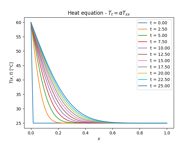
My suggestion would be to use an ODE solver combined with the method of lines instead of trying to use a non-linear system solver.

Here's an example of what this might look like:

import numpy as np
import matplotlib.pyplot as plt
from scipy.integrate import solve_ivp 

def F(t,y,alpha,dx):

    dydt = np.empty_like(y)
    alpha = alpha/dx**2

    # BC at x = 0
    dydt[0] = 0
    # BC at x = L
    dydt[-1] = 0
    # Interior nodes
    dydt[1:-1] = alpha*(y[2:] - 2*y[1:-1] + y[0:-2])

    return dydt

if __name__ == '__main__':
    
    t_max = 25
    alpha = 0.001
    N = 61

    x, dx = np.linspace(0,1,N,retstep=True)
    t = np.linspace(0,t_max,11)

    T0 = 25*np.ones_like(x)
    T0[0] = 60

    def F_(t,y):
        return F(t,y,alpha,dx)
        
    sol = solve_ivp(F_,(0,t_max),T0,method="LSODA",t_eval=t)

    plt.plot(x,sol.y)
    plt.xlabel(r"$x$")
    plt.ylabel(r"$T(x,t)$ [°C]")
    plt.title(r"Heat equation - $T_t = \alpha T_{xx}$")

    plt.legend(["t = {:0.2f}".format(t_) for t_ in t])

    plt.show()