Problem
I am using finite difference method to solve classic problem of flow around cylinder, for validation of my group's immersive boundary method.
The common way to validate numerical method is calculating drag and lift coefficient. But my result is far form other's results. So it must be error in my force calculation, and I don't know what is wrong.
Two resolution are tested:
Nx = Ny = 512, H = 1/64, dt = 1.8e-3, Nib = 100
Nx = Ny = 1024, H = 1/128, dt = 0.9e-3, Nib = 200
where Nx, Ny is grid size of staggered grid, it means that the pressure field's size if Nx * Ny, u component of velocity field is (Nx + 1) * Ny, v component of velocity field is Nx * (Ny + 1), Nib is the IB points number in cylinder virtual surface.
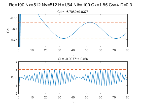
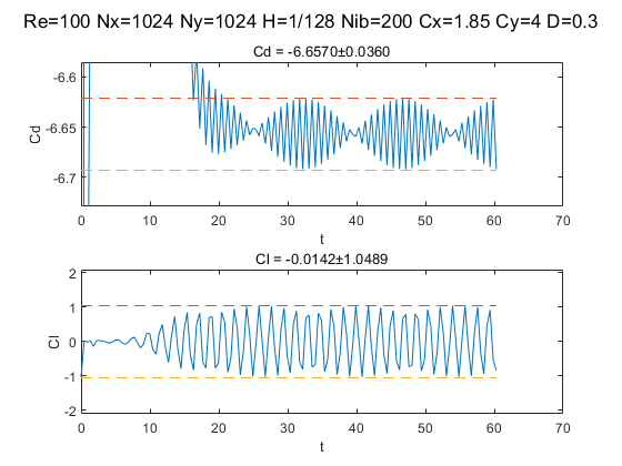
I have two method to calculate force, the result is shown by coefficient. The first method result:
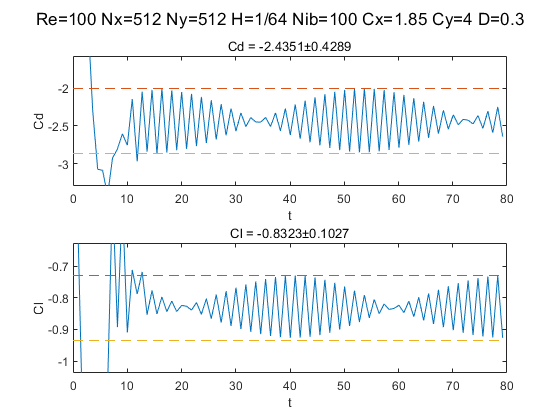
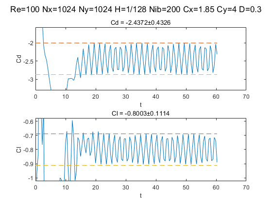
the second method:
As you can see, almost all results have violent oscillations. I don't know why.
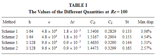
The correct result from
Lai, Ming-Chih, and Charles S. Peskin. "An immersed boundary method with formal second-order accuracy and reduced numerical viscosity." Journal of computational Physics 160.2 (2000): 705-719.
is
So you can see my result have grid independence, but method 1 result is several times the normal coefficient, method 2 have something wrong since its lift coefficient' s origin isn't 0.
I will show my solving pipeline below, thanks for any advice!
Drag and lift coefficient
Formula of lift coefficient:
$$ C_l = \dfrac{F_L}{qS} = \dfrac{F_L}{\frac{1}{2}\rho u^2 S} = \dfrac{2F_L}{\rho u^2 S}, $$
where $F_L$ is lift force, $\rho$ is fluid density, $u$ is inlet velocity, $S$ is reference surface.
Formula of drag coefficient:
$$ C_d = \dfrac{2F_D}{\rho u^2 S}, $$
where $F_D$ is lift force.
Calculating force
All my test here is the same setting: fluid domain size = [0, 8], cylinder center position = (1.85, 4), cylinder diameter D = 0.3, Re = 100, fluid density $\rho$ = 1, fluid inlet velocity $U$= 1, fluid dynamic viscosity $\mu$ is calculate according to Re.
Two resolution are tested:
Nx = Ny = 512, H = 1/64, dt = 1.8e-3, Nib = 100
Nx = Ny = 1024, H = 1/128, dt = 0.9e-3, Nib = 200
In code, it is configed by definition.
#define H          1.0 / 128.0
#define Nx         8.0 / (H)
#define Ny         8.0 / (H)
#define T_STEP     0.9e-3
#define MAX_STEP   100000
#define OUTPUT_GAP 500

#define CENTER_X 1.85
#define CENTER_Y 4
#define CY_R     0.15
#define CY_N     200

#define INLET_FLUID_VELOCITY 1.0
#define FLUID_DENSITY        1.0

#define REYNOLDS_NUM 100.0

#define DYNAMIC_VISCOSITY   FLUID_DENSITY* INLET_FLUID_VELOCITY* CY_R * 2.0 / REYNOLDS_NUM
#define KINEMATIC_VISCOSITY DYNAMIC_VISCOSITY / FLUID_DENSITY
To know the drag and lift force equals to calculating force of solid applied by fluid.
My methods are obtained from this paper:
Lai, Ming-Chih, and Charles S. Peskin. "An immersed boundary method with formal second-order accuracy and reduced numerical viscosity." Journal of computational Physics 160.2 (2000): 705-719.
I have tested two methods in this paper: One is directly sum up the IB force in all IB points, the other is using momentum conservation of NS equation.
The first method
$$ F_D = -\int_{\Omega}f_1 \mathrm{d} \mathbf{x} = -\int_0^{L_b}F_1 \mathrm{d}s, $$
$$ F_L = -\int_{\Omega}f_2 \mathrm{d} \mathbf{x} = -\int_0^{L_b}F_2 \mathrm{d}s, $$
where $F_D,F_L$ is drag force and lift force, $f_1, f_2$ is x and y component of IB force distributed to Euler grid, $F_1, F_2$ is x and y component of IB force at Lagrangian IB points. $\mathrm{d}\mathbf{x}$ seems like position of Euler grid, but it is annotation of the paper. I may think $\mathrm{d}\sigma$ looks nice, because it implies delta surface.
In code, to get the force, I sum up the IB force and then multiply it with h^2, h is interval length of IB points.
The second method:
NS equation in x component
$$ \dfrac{\partial u_1}{\partial t} + (\mathbf u \cdot \nabla)u_1 = -\dfrac{1}{\rho} \dfrac{\partial p}{\partial x} + \dfrac{\mu}{\rho}\nabla \cdot \nabla u_1 + f_1 $$
Integration form
$$ \dfrac{\partial}{\partial t}\int_{\Omega_0}\rho u_1 \mathrm{d} \mathbf x + \int_{\partial \Omega_0} \rho u_1 \mathbf u \cdot \mathbf n \mathrm{d} s = - \int_{\Omega_0} p n_1 \mathrm{d} \mathbf x + \int_{\partial \Omega_0} \mu (\dfrac{\partial u_1}{\partial x_j} + \dfrac{\partial u_j}{\partial x_1}) n_j \mathrm{d} s + \int_{\Omega_0} f_1 \mathrm{d} \mathbf x $$
When fluid become steady, the first term = 0, then
$$ \int_{\partial \Omega_0} \rho u_1 \mathbf u \cdot \mathbf n \mathrm{d} s = - \int_{\Omega_0} p n_1 \mathrm{d} \mathbf x + \int_{\partial \Omega_0} \mu (\dfrac{\partial u_1}{\partial x_j} + \dfrac{\partial u_j}{\partial x_1}) n_j \mathrm{d} s + \int_{\Omega_0} f_1 \mathrm{d} \mathbf x $$
Then drag force
$$ F_D = -\int_{\Omega_0} f_1 \mathrm{d} \mathbf x = -\int_{\partial \Omega_0} \rho u_1 \mathbf u \cdot \mathbf n \mathrm{d} s - \int_{\partial \Omega_0} p n_1 \mathrm{d} s + \int_{\partial \Omega_0} \mu (\dfrac{\partial u_1}{\partial x_j} + \dfrac{\partial u_j}{\partial x_1}) n_j \mathrm{d} s $$
lift force
$$ F_L = -\int_{\Omega_0} f_2 \mathrm{d} \mathbf x = -\int_{\partial \Omega_0} \rho u_2 \mathbf u \cdot \mathbf n \mathrm{d} s - \int_{\partial \Omega_0} p n_2 \mathrm{d} s + \int_{\partial \Omega_0} \mu (\dfrac{\partial u_2}{\partial x_j} + \dfrac{\partial u_j}{\partial x_2}) n_j \mathrm{d} s $$
Therefore, we simply pick any square domain $\Omega_0$ enclosing the cylinder and compute the line integrals of the above equation to obtain the drag force.
My code reproduction is:
#include "calc_solid_force_from_fluid.h"

double dudx(var& u, int i, int j, double h)
{
    double dudx = (u(i + 1, j) - u(i, j)) / h;
    return dudx;
}

double dudy(var& u, int i, int j, double h)
{
    double u_i_j_add_half         = 0.5 * (u(i, j) + u(i, j + 1));         // u(i, j + 1/2)
    double u_i_add_1_j_add_half   = 0.5 * (u(i + 1, j) + u(i + 1, j + 1)); // u(i + 1, j + 1/2)
    double u_i_j_minus_half       = 0.5 * (u(i, j) + u(i, j - 1));         // u(i, j - 1/2)
    double u_i_add_1_j_minus_half = 0.5 * (u(i + 1, j) + u(i + 1, j - 1)); // u(i + 1, j - 1/2)

    double u_i_add_half_j_add_half   = 0.5 * (u_i_j_add_half + u_i_add_1_j_add_half);     // u(i + 1/2, j + 1/2)
    double u_i_add_half_j_minus_half = 0.5 * (u_i_j_minus_half + u_i_add_1_j_minus_half); // u(i + 1/2, j - 1/2)

    double dudy = (u_i_add_half_j_add_half - u_i_add_half_j_minus_half) / h;

    return dudy;
}

double dvdy(var& v, int i, int j, double h)
{
    double dvdy = (v(i, j + 1) - v(i, j)) / h;
    return dvdy;
}

double dvdx(var& v, int i, int j, double h)
{
    double v_i_add_half_j         = 0.5 * (v(i, j) + v(i + 1, j));         // v(i + 1/2, j)
    double v_i_add_half_j_add_1   = 0.5 * (v(i, j + 1) + v(i + 1, j + 1)); // v(i + 1/2, j + 1)
    double v_i_minus_half_j       = 0.5 * (v(i, j) + v(i - 1, j));         // v(i - 1/2, j)
    double v_i_minus_half_j_add_1 = 0.5 * (v(i, j + 1) + v(i - 1, j + 1)); // v(i - 1/2, j + 1)

    double v_i_add_half_j_add_half   = 0.5 * (v_i_add_half_j + v_i_add_half_j_add_1);     // v(i + 1/2, j + 1/2)
    double v_i_minus_half_j_add_half = 0.5 * (v_i_minus_half_j + v_i_minus_half_j_add_1); // v(i - 1/2, j + 1/2)

    double dvdx = (v_i_add_half_j_add_half - v_i_minus_half_j_add_half) / h;

    return dvdx;
}

double integrand_x(var&           u,
                   var&           v,
                   Neumann_field& p,
                   int            i,
                   int            j,
                   double         rho,
                   double         dynamic_viscosity,
                   double         h,
                   double         n1,
                   double         n2)
{
    double Fx = 0.0;

    Fx += -rho * u(i, j) * (u(i, j) * n1 + v(i, j) * n2);
    Fx += -p(i, j) * n1;
    Fx += dynamic_viscosity * (2.0 * dudx(u, i, j, h) * n1 + (dudy(u, i, j, h) + dvdx(v, i, j, h)) * n2);

    return Fx;
}

double integrand_y(var&           u,
                   var&           v,
                   Neumann_field& p,
                   int            i,
                   int            j,
                   double         rho,
                   double         dynamic_viscosity,
                   double         h,
                   double         n1,
                   double         n2)
{
    double Fy = 0.0;

    Fy += -rho * v(i, j) * (u(i, j) * n1 + v(i, j) * n2);
    Fy += -p(i, j) * n2;
    Fy += dynamic_viscosity * (2.0 * dvdy(v, i, j, h) * n2 + (dudy(u, i, j, h) + dvdx(v, i, j, h)) * n1);

    return Fy;
}

std::tuple<double, double> calc_solid_force_from_fluid(NSSolver2D& ns_solver,
                                                       double      rho,
                                                       double      dynamic_viscosity,
                                                       double      xmin,
                                                       double      xmax,
                                                       double      ymin,
                                                       double      ymax)
{
    var&           u = ns_solver.u;
    var&           v = ns_solver.v;
    Neumann_field& p = ns_solver.p;

    double h = ns_solver.h;

    // u

    int ixmin = int(xmin / ns_solver.h);
    int ixmax = int(xmax / ns_solver.h);
    int iymin = int(xmin / ns_solver.h - 0.5);
    int iymax = int(xmax / ns_solver.h - 0.5);

    double Fx = 0.0, Fy = 0.0;

    // Fx

    // left
    for (int i = ixmin, j = iymin; j < iymax; j++)
    {
        Fx += integrand_x(u, v, p, i, j, rho, dynamic_viscosity, h, -1.0, 0.0);
    }

    // right
    for (int i = ixmax, j = iymin; j < iymax; j++)
    {
        Fx += integrand_x(u, v, p, i, j, rho, dynamic_viscosity, h, 1.0, 0.0);
    }

    // down
    for (int i = ixmin, j = iymin; i < ixmax; i++)
    {
        Fx += integrand_x(u, v, p, i, j, rho, dynamic_viscosity, h, 0.0, -1.0);
    }

    // up
    for (int i = ixmin, j = iymax; i < ixmax; i++)
    {
        Fx += integrand_x(u, v, p, i, j, rho, dynamic_viscosity, h, 0.0, 1.0);
    }

    // Fy

    ixmin = int(xmin / ns_solver.h - 0.5);
    ixmax = int(xmax / ns_solver.h - 0.5);
    iymin = int(xmin / ns_solver.h);
    iymax = int(xmax / ns_solver.h);

    // left
    for (int i = ixmin, j = iymin; j < iymax; j++)
    {
        Fy += integrand_y(u, v, p, i, j, rho, dynamic_viscosity, h, -1.0, 0.0);
    }

    // right
    for (int i = ixmax, j = iymin; j < iymax; j++)
    {
        Fy += integrand_y(u, v, p, i, j, rho, dynamic_viscosity, h, 1.0, 0.0);
    }

    // down
    for (int i = ixmin, j = iymin; i < ixmax; i++)
    {
        Fy += integrand_y(u, v, p, i, j, rho, dynamic_viscosity, h, 0.0, -1.0);
    }

    // up
    for (int i = ixmin, j = iymax; i < ixmax; i++)
    {
        Fy += integrand_y(u, v, p, i, j, rho, dynamic_viscosity, h, 0.0, 1.0);
    }

    Fx *= h; // ds in line integrals
    Fy *= h; // ds in line integrals

    return {Fx, Fy};
}
The code directly return what the force I need.
The code consider two main aspects:
There is transform from world space
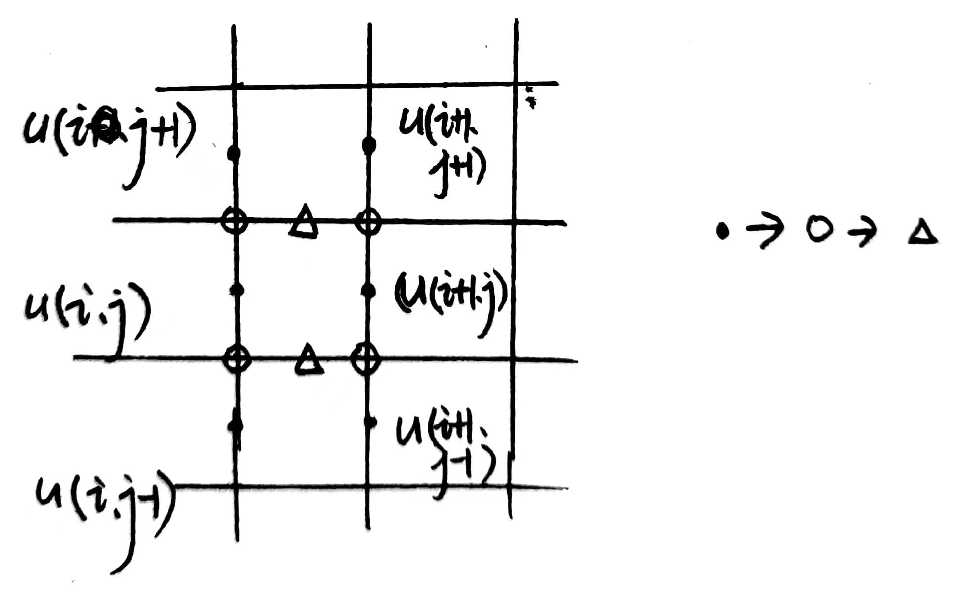
xmin, xmaxto index spaceixmin, ixmax, which is related with staggered grid.To get the
dudy, dvdxin staggered grid, I interpolate theu, vas figure below.
Other details about solver implementation
SIMPLE algorithm
The solving algorithm of NS equation is SIMPLE algorithm.
for (int time_iter = 0; time_iter < MAX_STEP; time_iter++)
{
    _NS_solver.apply_boundary();
    _NS_solver.cal_conv();
    _NS_solver.apply_pressure_gredient();
    _NS_solver.u2F(cylinder);
    _NS_solver.apply_ib_force(cylinder);
    _NS_solver.apply_boundary();
    _NS_solver.refresh_vars();

    std::cout << "PPE" << std::endl;
    for (int corr_iter = 0; corr_iter < 1; corr_iter++)
    {
        _NS_solver.cal_divu();
        _PE_solver.solve(_NS_solver.Div_u, _NS_solver.p);
        _NS_solver.apply_pressure_gredient();
    }

    ...
}
More specific details can't be provided because they are contributions of our groups, but I think the pipeline is enough.
Immersive boundary model
There are many models of immersive boundary method, what we used is "direct forcing" model, basically it means that the IB force is evaluated by the difference between the actual velocity of solid and the fluid velocity in solid position.
$$ \mathbf{F}(\mathbf{X}_l^{(m)}) = \dfrac{\mathbf{U}^{(d)}(\mathbf{X}_l) - \widetilde{\mathbf{U}}(\mathbf{X}_l)}{\Delta t} \forall l;m, $$
More information see:
Uhlmann, Markus. "An immersed boundary method with direct forcing for the simulation of particulate flows." Journal of computational physics 209.2 (2005): 448-476.
