Post Closed as "Not suitable for this site" by Bill Barth, Brian Borchers, Wolfgang Bangerth, Christian Clason, Paul

FEniCs: help in implementimplementing the boundary condition for 1D problem

I have just startingstarted learning FEniCS and have used: http://www.scientificpython.net/pyblog/fenics-linear-two-point-bvp to write a script for solving:

           u'' + u = 1
             
           u(0) = 1, u'(1) = 0

with exact solution,

           u(x) = exp(-x)/ exp(-1) + x + ( -1+exp(-1) )/ exp(-1)

Clearly the weak formulation of the above problem is:

           -(u', v') + (u,v) = (g,v) ; with g = 1

Here is the edited code:

    from dolfin import *

    # definig mesh
    mesh = IntervalMesh(20, 0, 1)

    # definig Function space on this mesh using Lagrange polynoimals of degree 2.
    V = FunctionSpace(mesh, "CG", 2)


    # definign boundary values
    #u0 = Constant(0)
    u0 = Expression("x[0]")

    # this functions checks whether the input x is on the boundary or not.
    def DirichletBoundary(x, on_boundary):
         tol = 1e-14
         return on_boundary and abs(x < tol)

     # Enforcing u = u0 at x = 0
     bc = DirichletBC(V, u0, DirichletBoundary)

     # Setting up the variational problem
     u = TrialFunction(V)
     v = TestFunction(V)
     f = Constant(1)
     g = Constant(1)
     a = -inner(grad(u), grad(v))*dx + inner(u,v)*dx
     L = f*v*dx

     # solving the variational problem.
     u = Function(V)
     solve( a == L, u, bc)

     # plotting solution
     plot(u, interactive = True)

Clearly the solution plot does not incorporate the boundary condition u(0) = 1. enter image description here
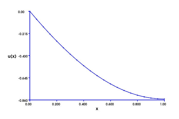
Would any body please help?

FEniCs: help in implement the boundary condition for 1D problem

I have just starting learning FEniCS and have used: http://www.scientificpython.net/pyblog/fenics-linear-two-point-bvp to write a script for solving:

           u'' + u = 1
             
           u(0) = 1, u'(1) = 0

with exact solution,

           u(x) = exp(-x)/ exp(-1) + x + ( -1+exp(-1) )/ exp(-1)

Clearly the weak formulation of the above problem is:

           -(u', v') + (u,v) = (g,v) ; with g = 1

Here is the edited code:

    from dolfin import *

    # definig mesh
    mesh = IntervalMesh(20, 0, 1)

    # definig Function space on this mesh using Lagrange polynoimals of degree 2.
    V = FunctionSpace(mesh, "CG", 2)


    # definign boundary values
    #u0 = Constant(0)
    u0 = Expression("x[0]")

    # this functions checks whether the input x is on the boundary or not.
    def DirichletBoundary(x, on_boundary):
         tol = 1e-14
         return on_boundary and abs(x < tol)

     # Enforcing u = u0 at x = 0
     bc = DirichletBC(V, u0, DirichletBoundary)

     # Setting up the variational problem
     u = TrialFunction(V)
     v = TestFunction(V)
     f = Constant(1)
     g = Constant(1)
     a = -inner(grad(u), grad(v))*dx + inner(u,v)*dx
     L = f*v*dx

     # solving the variational problem.
     u = Function(V)
     solve( a == L, u, bc)

     # plotting solution
     plot(u, interactive = True)

Clearly the solution plot does not incorporate the boundary condition u(0) = 1. enter image description here

Would any body please help?

FEniCs: help in implementing the boundary condition for 1D problem

I have just started learning FEniCS and have used: http://www.scientificpython.net/pyblog/fenics-linear-two-point-bvp to write a script for solving:

           u'' + u = 1
             
           u(0) = 1, u'(1) = 0

with exact solution,

           u(x) = exp(-x)/ exp(-1) + x + ( -1+exp(-1) )/ exp(-1)

Clearly the weak formulation of the above problem is:

           -(u', v') + (u,v) = (g,v) ; with g = 1

Here is the edited code:

    from dolfin import *

    # definig mesh
    mesh = IntervalMesh(20, 0, 1)

    # definig Function space on this mesh using Lagrange polynoimals of degree 2.
    V = FunctionSpace(mesh, "CG", 2)


    # definign boundary values
    #u0 = Constant(0)
    u0 = Expression("x[0]")

    # this functions checks whether the input x is on the boundary or not.
    def DirichletBoundary(x, on_boundary):
         tol = 1e-14
         return on_boundary and abs(x < tol)

     # Enforcing u = u0 at x = 0
     bc = DirichletBC(V, u0, DirichletBoundary)

     # Setting up the variational problem
     u = TrialFunction(V)
     v = TestFunction(V)
     f = Constant(1)
     g = Constant(1)
     a = -inner(grad(u), grad(v))*dx + inner(u,v)*dx
     L = f*v*dx

     # solving the variational problem.
     u = Function(V)
     solve( a == L, u, bc)

     # plotting solution
     plot(u, interactive = True)

Clearly the solution plot does not incorporate the boundary condition u(0) = 1. enter image description here

Would any body please help?

Source Link
Sohail
  • 246
  • 1
  • 6

FEniCs: help in implement the boundary condition for 1D problem

I have just starting learning FEniCS and have used: http://www.scientificpython.net/pyblog/fenics-linear-two-point-bvp to write a script for solving:

           u'' + u = 1
             
           u(0) = 1, u'(1) = 0

with exact solution,

           u(x) = exp(-x)/ exp(-1) + x + ( -1+exp(-1) )/ exp(-1)

Clearly the weak formulation of the above problem is:

           -(u', v') + (u,v) = (g,v) ; with g = 1

Here is the edited code:

    from dolfin import *

    # definig mesh
    mesh = IntervalMesh(20, 0, 1)

    # definig Function space on this mesh using Lagrange polynoimals of degree 2.
    V = FunctionSpace(mesh, "CG", 2)


    # definign boundary values
    #u0 = Constant(0)
    u0 = Expression("x[0]")

    # this functions checks whether the input x is on the boundary or not.
    def DirichletBoundary(x, on_boundary):
         tol = 1e-14
         return on_boundary and abs(x < tol)

     # Enforcing u = u0 at x = 0
     bc = DirichletBC(V, u0, DirichletBoundary)

     # Setting up the variational problem
     u = TrialFunction(V)
     v = TestFunction(V)
     f = Constant(1)
     g = Constant(1)
     a = -inner(grad(u), grad(v))*dx + inner(u,v)*dx
     L = f*v*dx

     # solving the variational problem.
     u = Function(V)
     solve( a == L, u, bc)

     # plotting solution
     plot(u, interactive = True)

Clearly the solution plot does not incorporate the boundary condition u(0) = 1. enter image description here

Would any body please help?