Mod Moved Comments To Chat
added 76 characters in body
Source Link
knl
  • 2.1k
  • 12
  • 17

You would need to linearize the problem. I prefer to do it before discretization but it's possible to do also after discretization. (I'm a bit skeptical of linearization after discretization because I have never looked into the details. In general, discretization and linearization steps do not commute.)

In the following I assume that the equation is actually $\partial_t u = \partial_x(a(u) \partial_x u)$ and that you have the boundary condition $u=0$.

The weak form is $$(\partial_t u, v) = -(a(u) \partial_x u, \partial_x v).$$ I prefer to first do the time discretization so that you see the structure of the resulting problem. E.g., implicit Euler method leads to $$(\delta^{-1}(u_n - u_{n-1}), v) = -(a(u_n) \partial_x u_n, \partial_x v),$$ or, equivalently, $$(\delta^{-1} u_n, v) + (a(u_n) \partial_x u_n, \partial_x v) = (\delta^{-1}u_{n-1}, v),$$ where $n$ runs over the time steps and $\delta > 0$ is the size of the step. The equation is still nonlinear in $u_n$ and you must linearize. One option is to do a fixed-point iteration (inside each time step $n$) by repeatedly finding $u_{k,n}$ from $$(\delta^{-1} u_{k,n}, v) + (a(u_{k-1,n}) \partial_x u_{k,n}, \partial_x v) = (\delta^{-1}u_{n-1}, v),$$ where $k$ runs over the linearization steps and $u_{k-1,n}$ is the function from the previous iteration. Notice how you now have two iterations: one for time discretization and one for linearization.

I made an example case with $u(x) = \sin(\pi x)$ and solved it using the code I know the best (i.e. my own, you can install it in Python using pip install scikit-fem==2.0.0 if you want to run it):

from skfem import *
from skfem.helpers import *
from skfem.visuals.matplotlib import *
import numpy as np

m = MeshLine(); m.refine(5)
basis = InteriorBasis(m, ElementLineP1ElementLineP2())
a = lambda w: (1. * w) ** 2
bilinf_stiffness = BilinearForm(lambda u, v, w: a(w['u_prev']) * dot(grad(u), grad(v)))
delta = 0.101
M = BilinearForm(lambda u, v, w: 1. / delta * u * v).assemble(basis)
load = LinearForm(lambda v, w: 1. / delta * w['u_prev'] * v)

u = project(lambda x: np.sin(np.pi * m.p[0]x[0]), basis_to=basis)
plot(mbasis, u)
for n in range(10100): # 10100 time steps 
    b = load.assemble(basis, u_prev=basis.interpolate(u))
    for k in range(250): # 250 linearization loops 
        A = bilinf_stiffness.assemble(basis, u_prev=basis.interpolate(u))
        b = load.assemble(basis, u_prev=basis.interpolate(u))
        u = solve(*condense(A + M, b, D=m.boundary_nodes()))
    print("iteration {}".format(n))
plot(mbasis, u);  
show()

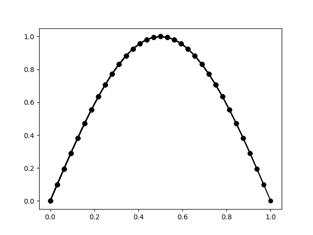
This gives the following two pictures (initial condition and the result at $t=1$): Initial field Solution at t=1Solution at t=1
There are obviously lots of alternative ways of doing this, but this should give you the general idea.

You would need to linearize the problem. I prefer to do it before discretization but it's possible to do also after discretization. (I'm a bit skeptical of linearization after discretization because I have never looked into the details. In general, discretization and linearization steps do not commute.)

In the following I assume that the equation is actually $\partial_t u = \partial_x(a(u) \partial_x u)$ and that you have the boundary condition $u=0$.

The weak form is $$(\partial_t u, v) = -(a(u) \partial_x u, \partial_x v).$$ I prefer to first do the time discretization so that you see the structure of the resulting problem. E.g., implicit Euler method leads to $$(\delta^{-1}(u_n - u_{n-1}), v) = -(a(u_n) \partial_x u_n, \partial_x v),$$ or, equivalently, $$(\delta^{-1} u_n, v) + (a(u_n) \partial_x u_n, \partial_x v) = (\delta^{-1}u_{n-1}, v),$$ where $n$ runs over the time steps and $\delta > 0$ is the size of the step. The equation is still nonlinear in $u_n$ and you must linearize. One option is to do a fixed-point iteration (inside each time step $n$) by repeatedly finding $u_{k,n}$ from $$(\delta^{-1} u_{k,n}, v) + (a(u_{k-1,n}) \partial_x u_{k,n}, \partial_x v) = (\delta^{-1}u_{n-1}, v),$$ where $k$ runs over the linearization steps and $u_{k-1,n}$ is the function from the previous iteration. Notice how you now have two iterations: one for time discretization and one for linearization.

I made an example case with $u(x) = \sin(\pi x)$ and solved it using the code I know the best (i.e. my own, you can install it in Python using pip install scikit-fem==2.0.0 if you want to run it):

from skfem import *
from skfem.helpers import *
from skfem.visuals.matplotlib import *
import numpy as np

m = MeshLine(); m.refine(5)
basis = InteriorBasis(m, ElementLineP1())
a = lambda w: (1. * w) ** 2
bilinf_stiffness = BilinearForm(lambda u, v, w: a(w['u_prev']) * dot(grad(u), grad(v)))
delta = 0.1
M = BilinearForm(lambda u, v, w: 1. / delta * u * v).assemble(basis)
load = LinearForm(lambda v, w: 1. / delta * w['u_prev'] * v)

u = np.sin(np.pi * m.p[0])
plot(m, u)
for n in range(10): # 10 time steps 
    for k in range(250): # 250 linearization loops 
        A = bilinf_stiffness.assemble(basis, u_prev=basis.interpolate(u))
        b = load.assemble(basis, u_prev=basis.interpolate(u))
        u = solve(*condense(A + M, b, D=m.boundary_nodes()))
plot(m, u); show()

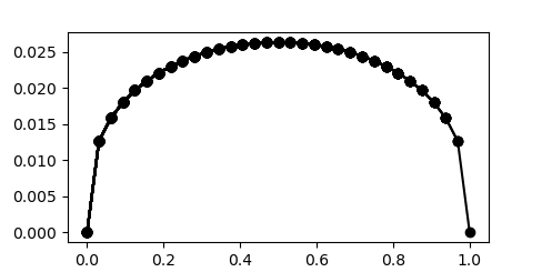
This gives the following two pictures (initial condition and the result at $t=1$): Initial field Solution at t=1
There are obviously lots of alternative ways of doing this, but this should give you the general idea.

You would need to linearize the problem. I prefer to do it before discretization but it's possible to do also after discretization. (I'm a bit skeptical of linearization after discretization because I have never looked into the details. In general, discretization and linearization steps do not commute.)

In the following I assume that the equation is actually $\partial_t u = \partial_x(a(u) \partial_x u)$ and that you have the boundary condition $u=0$.

The weak form is $$(\partial_t u, v) = -(a(u) \partial_x u, \partial_x v).$$ I prefer to first do the time discretization so that you see the structure of the resulting problem. E.g., implicit Euler method leads to $$(\delta^{-1}(u_n - u_{n-1}), v) = -(a(u_n) \partial_x u_n, \partial_x v),$$ or, equivalently, $$(\delta^{-1} u_n, v) + (a(u_n) \partial_x u_n, \partial_x v) = (\delta^{-1}u_{n-1}, v),$$ where $n$ runs over the time steps and $\delta > 0$ is the size of the step. The equation is still nonlinear in $u_n$ and you must linearize. One option is to do a fixed-point iteration (inside each time step $n$) by repeatedly finding $u_{k,n}$ from $$(\delta^{-1} u_{k,n}, v) + (a(u_{k-1,n}) \partial_x u_{k,n}, \partial_x v) = (\delta^{-1}u_{n-1}, v),$$ where $k$ runs over the linearization steps and $u_{k-1,n}$ is the function from the previous iteration. Notice how you now have two iterations: one for time discretization and one for linearization.

I made an example case with $u(x) = \sin(\pi x)$ and solved it using the code I know the best (i.e. my own, you can install it in Python using pip install scikit-fem==2.0.0 if you want to run it):

from skfem import *
from skfem.helpers import *
from skfem.visuals.matplotlib import *
import numpy as np

m = MeshLine(); m.refine(5)
basis = InteriorBasis(m, ElementLineP2())
a = lambda w: (1. * w) ** 2
bilinf_stiffness = BilinearForm(lambda u, v, w: a(w['u_prev']) * dot(grad(u), grad(v)))
delta = 0.01
M = BilinearForm(lambda u, v, w: 1. / delta * u * v).assemble(basis)
load = LinearForm(lambda v, w: 1. / delta * w['u_prev'] * v)

u = project(lambda x: np.sin(np.pi * x[0]), basis_to=basis)
plot(basis, u)
for n in range(100): # 100 time steps 
    b = load.assemble(basis, u_prev=basis.interpolate(u))
    for k in range(250): # 250 linearization loops
        A = bilinf_stiffness.assemble(basis, u_prev=basis.interpolate(u))
        u = solve(*condense(A + M, b, D=m.boundary_nodes()))
    print("iteration {}".format(n))
plot(basis, u) 
show()

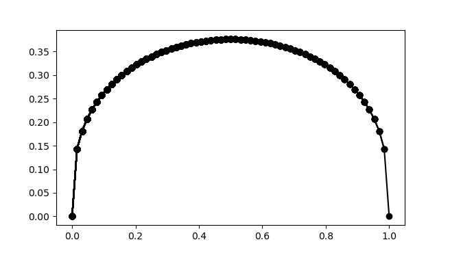
This gives the following two pictures (initial condition and the result at $t=1$): Initial field Solution at t=1
There are obviously lots of alternative ways of doing this, but this should give you the general idea.
deleted 7 characters in body
Source Link
knl
  • 2.1k
  • 12
  • 17

You would need to linearize the problem. I prefer to do it before discretization but it's possible to do also after discretization. (I'm a bit skeptical of linearization after discretization because I have never looked into the details. In general, discretization and linearization steps do not commute.)

In the following I assume that the equation is actually $\partial_t u = \partial_x(a(u) \partial_x u)$ and that you have the boundary condition $u=0$.

The weak form is $$(\partial_t u, v) = -(a(u) \partial_x u, \partial_x v).$$ I prefer to first do the time discretization so that you see the structure of the resulting problem. E.g., implicit Euler method leads to $$(\delta^{-1}(u_n - u_{n-1}), v) = -(a(u_n) \partial_x u_n, \partial_x v),$$ or, equivalently, $$(\delta^{-1} u_n, v) + (a(u_n) \partial_x u_n, \partial_x v) = (\delta^{-1}u_{n-1}, v),$$ where $n$ runs over the time steps and $\delta > 0$ is the size of the step. The equation is still nonlinear in $u_n$ and you must linearize. One option is to do a fixed-point iteration (inside each time step $n$) by repeatedly finding $u_{k,n}$ from $$(\delta^{-1} u_{k,n}, v) + (a(u_{k-1,n}) \partial_x u_{k,n}, \partial_x v) = (\delta^{-1}u_{n-1}, v),$$ where $k$ runs over the linearization steps and $u_{k-1,n}$ is the function from the previous iteration. Notice how you now have two iterations: one for time discretization and one for linearization.

I made an example case with $u(x) = \sin(\pi x)$ and solved it using the code I know the best (i.e. my own, you can install it in Python using pip install scikit-fem==2.0.0 if you want to run it):

from skfem import *
from skfem.helpers import *
from skfem.visuals.matplotlib import *
import numpy as np

m = MeshLine(); m.refine(5)
basis = InteriorBasis(m, ElementLineP1())
a = lambda w: (1. * w) ** 2
bilinf_stiffness = BilinearForm(lambda u, v, w: a(w['u_prev']) * dot(grad(u), grad(v)))
delta = 0.1
M = BilinearForm(lambda u, v, w: 1. / delta * u * v).assemble(basis)
load = LinearForm(lambda v, w: 1. / delta * w['u_prev'] * v)

u = np.sin(np.pi * m.p[0])
plot(m, u)
for n in range(10): # 10 time steps 
    for k in range(8250): # 8250 linearization loops 
        A = bilinf_stiffness.assemble(basis, u_prev=basis.interpolate(u))
        b = load.assemble(basis, u_prev=basis.interpolate(u))
        u = solve(*condense(A + M, b, D=m.boundary_nodes()))
plot(m, u); show()

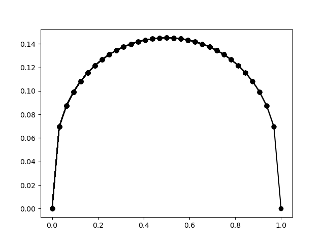
This gives the following two pictures (initial condition and the result at $t=1$): Initial field enter image description hereSolution at t=1

There are obviously lots of alternative ways of doing this, but this should give you the general idea.

You would need to linearize the problem. I prefer to do it before discretization but it's possible to do also after discretization. (I'm a bit skeptical of linearization after discretization because I have never looked into the details. In general, discretization and linearization steps do not commute.)

In the following I assume that the equation is actually $\partial_t u = \partial_x(a(u) \partial_x u)$ and that you have the boundary condition $u=0$.

The weak form is $$(\partial_t u, v) = -(a(u) \partial_x u, \partial_x v).$$ I prefer to first do the time discretization so that you see the structure of the resulting problem. E.g., implicit Euler method leads to $$(\delta^{-1}(u_n - u_{n-1}), v) = -(a(u_n) \partial_x u_n, \partial_x v),$$ or, equivalently, $$(\delta^{-1} u_n, v) + (a(u_n) \partial_x u_n, \partial_x v) = (\delta^{-1}u_{n-1}, v),$$ where $n$ runs over the time steps and $\delta > 0$ is the size of the step. The equation is still nonlinear in $u_n$ and you must linearize. One option is to do a fixed-point iteration (inside each time step $n$) by repeatedly finding $u_{k,n}$ from $$(\delta^{-1} u_{k,n}, v) + (a(u_{k-1,n}) \partial_x u_{k,n}, \partial_x v) = (\delta^{-1}u_{n-1}, v),$$ where $k$ runs over the linearization steps and $u_{k-1,n}$ is the function from the previous iteration. Notice how you now have two iterations: one for time discretization and one for linearization.

I made an example case with $u(x) = \sin(\pi x)$ and solved it using the code I know the best (i.e. my own, you can install it in Python using pip install scikit-fem==2.0.0 if you want to run it):

from skfem import *
from skfem.helpers import *
from skfem.visuals.matplotlib import *
import numpy as np

m = MeshLine(); m.refine(5)
basis = InteriorBasis(m, ElementLineP1())
a = lambda w: (1. * w) ** 2
bilinf_stiffness = BilinearForm(lambda u, v, w: a(w['u_prev']) * dot(grad(u), grad(v)))
delta = 0.1
M = BilinearForm(lambda u, v, w: 1. / delta * u * v).assemble(basis)
load = LinearForm(lambda v, w: 1. / delta * w['u_prev'] * v)

u = np.sin(np.pi * m.p[0])
plot(m, u)
for n in range(10): # 10 time steps 
    for k in range(8): # 8 linearization loops 
        A = bilinf_stiffness.assemble(basis, u_prev=basis.interpolate(u))
        b = load.assemble(basis, u_prev=basis.interpolate(u))
        u = solve(*condense(A + M, b, D=m.boundary_nodes()))
plot(m, u); show()

This gives the following two pictures (initial condition and the result at $t=1$): Initial field enter image description here

There are obviously lots of alternative ways of doing this, but this should give you the general idea.

You would need to linearize the problem. I prefer to do it before discretization but it's possible to do also after discretization. (I'm a bit skeptical of linearization after discretization because I have never looked into the details. In general, discretization and linearization steps do not commute.)

In the following I assume that the equation is actually $\partial_t u = \partial_x(a(u) \partial_x u)$ and that you have the boundary condition $u=0$.

The weak form is $$(\partial_t u, v) = -(a(u) \partial_x u, \partial_x v).$$ I prefer to first do the time discretization so that you see the structure of the resulting problem. E.g., implicit Euler method leads to $$(\delta^{-1}(u_n - u_{n-1}), v) = -(a(u_n) \partial_x u_n, \partial_x v),$$ or, equivalently, $$(\delta^{-1} u_n, v) + (a(u_n) \partial_x u_n, \partial_x v) = (\delta^{-1}u_{n-1}, v),$$ where $n$ runs over the time steps and $\delta > 0$ is the size of the step. The equation is still nonlinear in $u_n$ and you must linearize. One option is to do a fixed-point iteration (inside each time step $n$) by repeatedly finding $u_{k,n}$ from $$(\delta^{-1} u_{k,n}, v) + (a(u_{k-1,n}) \partial_x u_{k,n}, \partial_x v) = (\delta^{-1}u_{n-1}, v),$$ where $k$ runs over the linearization steps and $u_{k-1,n}$ is the function from the previous iteration. Notice how you now have two iterations: one for time discretization and one for linearization.

I made an example case with $u(x) = \sin(\pi x)$ and solved it using the code I know the best (i.e. my own, you can install it in Python using pip install scikit-fem==2.0.0 if you want to run it):

from skfem import *
from skfem.helpers import *
from skfem.visuals.matplotlib import *
import numpy as np

m = MeshLine(); m.refine(5)
basis = InteriorBasis(m, ElementLineP1())
a = lambda w: (1. * w) ** 2
bilinf_stiffness = BilinearForm(lambda u, v, w: a(w['u_prev']) * dot(grad(u), grad(v)))
delta = 0.1
M = BilinearForm(lambda u, v, w: 1. / delta * u * v).assemble(basis)
load = LinearForm(lambda v, w: 1. / delta * w['u_prev'] * v)

u = np.sin(np.pi * m.p[0])
plot(m, u)
for n in range(10): # 10 time steps 
    for k in range(250): # 250 linearization loops 
        A = bilinf_stiffness.assemble(basis, u_prev=basis.interpolate(u))
        b = load.assemble(basis, u_prev=basis.interpolate(u))
        u = solve(*condense(A + M, b, D=m.boundary_nodes()))
plot(m, u); show()

This gives the following two pictures (initial condition and the result at $t=1$): Initial field Solution at t=1

There are obviously lots of alternative ways of doing this, but this should give you the general idea.

added 90 characters in body
Source Link
knl
  • 2.1k
  • 12
  • 17

You would need to linearize the problem. I prefer to do it before discretization but it's possible to do also after discretization. (I'm a bit skeptical of linearization after discretization because I have never looked into the details. In general, discretization and linearization steps do not commute.)

In the following I assume that the equation is actually $\partial_t u = \partial_x(a(u) \partial_x u)$ and that you have the boundary condition $u=0$.

The weak form is $$(\partial_t u, v) = -(a(u) \partial_x u, \partial_x v).$$ I prefer to first do the time discretization so that you see the structure of the resulting problem. E.g., implicit Euler method leads to $$(\delta^{-1}(u_n - u_{n-1}), v) = -(a(u_n) \partial_x u_n, \partial_x v),$$ or, equivalently, $$(\delta^{-1} u_n, v) + (a(u_n) \partial_x u_n, \partial_x v) = (\delta^{-1}u_{n-1}, v),$$ where $n$ runs over the time steps and $\delta > 0$ is the size of the step. The equation is still nonlinear in $u_n$ and you must linearize. One option is to do a fixed-point iteration (inside each time step $n$) by repeatedly finding $u_{k,n}$ from $$(\delta^{-1} u_{k,n}, v) + (a(u_{k-1,n}) \partial_x u_{k,n}, \partial_x v) = (\delta^{-1}u_{n-1}, v),$$ where $k$ runs over the linearization steps and $u_{k-1,n}$ is the function from the previous iteration. Notice how you now have two iterations: one for time discretization and one for linearization.

I made an example case with $u(x) = \sin(\pi x)$ and solved it using the code I know the best (i.e. my own, you can install it in Python using pip install scikit-fem==2.0.0 if you want to run it):

from skfem import *
from skfem.helpers import *
from skfem.visuals.matplotlib import *
import numpy as np

m = MeshLine(); m.refine(5)
basis = InteriorBasis(m, ElementLineP1())
a = lambda w: (1. * w) ** 2
bilinf_stiffness = BilinearForm(lambda u, v, w: a(w['u_prev']) * dot(grad(u), grad(v)))
delta = 0.1
M = BilinearForm(lambda u, v, w: 1. / delta * u * v).assemble(basis)
load = LinearForm(lambda v, w: 1. / delta * w['u_prev'] * v)

u = np.sin(np.pi * m.p[0])
plot(m, u)
for n in range(10): # 10 time steps 
    for k in range(8): # 8 linearization loops 
        A = bilinf_stiffness.assemble(basis, u_prev=basis.interpolate(u))
        b = load.assemble(basis, u_prev=basis.interpolate(u))
        u = solve(*condense(A + M, b, D=m.boundary_nodes()))
plot(m, u); show()

This gives the following two pictures (initial condition and the result at $t=1$): Initial field enter image description here

There are obviously lots of alternative ways of doing this, but this should getgive you startedthe general idea.

You would need to linearize the problem. I prefer to do it before discretization but it's possible to do also after discretization. (I'm a bit skeptical of linearization after discretization because I have never looked into the details. In general, discretization and linearization steps do not commute.)

In the following I assume that the equation is actually $\partial_t u = \partial_x(a(u) \partial_x u)$ and that you have the boundary condition $u=0$.

The weak form is $$(\partial_t u, v) = -(a(u) \partial_x u, \partial_x v).$$ I prefer to first do the time discretization so that you see the structure of the resulting problem. E.g., implicit Euler method leads to $$(\delta^{-1}(u_n - u_{n-1}), v) = -(a(u_n) \partial_x u_n, \partial_x v),$$ or, equivalently, $$(\delta^{-1} u_n, v) + (a(u_n) \partial_x u_n, \partial_x v) = (\delta^{-1}u_{n-1}, v),$$ where $n$ runs over the time steps and $\delta > 0$ is the size of the step. The equation is still nonlinear in $u_n$ and you must linearize. One option is to do a fixed-point iteration (inside each time step $n$) by repeatedly finding $u_{k,n}$ from $$(\delta^{-1} u_{k,n}, v) + (a(u_{k-1,n}) \partial_x u_{k,n}, \partial_x v) = (\delta^{-1}u_{n-1}, v),$$ where $k$ runs over the linearization steps and $u_{k-1,n}$ is the function from the previous iteration. Notice how you now have two iterations: one for time discretization and one for linearization.

I made an example case with $u(x) = \sin(\pi x)$ and solved it using the code I know the best (i.e. my own):

from skfem import *
from skfem.helpers import *
from skfem.visuals.matplotlib import *
import numpy as np

m = MeshLine(); m.refine(5)
basis = InteriorBasis(m, ElementLineP1())
a = lambda w: (1. * w) ** 2
bilinf_stiffness = BilinearForm(lambda u, v, w: a(w['u_prev']) * dot(grad(u), grad(v)))
delta = 0.1
M = BilinearForm(lambda u, v, w: 1. / delta * u * v).assemble(basis)
load = LinearForm(lambda v, w: 1. / delta * w['u_prev'] * v)

u = np.sin(np.pi * m.p[0])
plot(m, u)
for n in range(10): # 10 time steps 
    for k in range(8): # 8 linearization loops 
        A = bilinf_stiffness.assemble(basis, u_prev=basis.interpolate(u))
        b = load.assemble(basis, u_prev=basis.interpolate(u))
        u = solve(*condense(A + M, b, D=m.boundary_nodes()))
plot(m, u); show()

This gives the following two pictures (initial condition and the result at $t=1$): Initial field enter image description here

There are obviously lots of alternative ways of doing this, but this should get you started.

You would need to linearize the problem. I prefer to do it before discretization but it's possible to do also after discretization. (I'm a bit skeptical of linearization after discretization because I have never looked into the details. In general, discretization and linearization steps do not commute.)

In the following I assume that the equation is actually $\partial_t u = \partial_x(a(u) \partial_x u)$ and that you have the boundary condition $u=0$.

The weak form is $$(\partial_t u, v) = -(a(u) \partial_x u, \partial_x v).$$ I prefer to first do the time discretization so that you see the structure of the resulting problem. E.g., implicit Euler method leads to $$(\delta^{-1}(u_n - u_{n-1}), v) = -(a(u_n) \partial_x u_n, \partial_x v),$$ or, equivalently, $$(\delta^{-1} u_n, v) + (a(u_n) \partial_x u_n, \partial_x v) = (\delta^{-1}u_{n-1}, v),$$ where $n$ runs over the time steps and $\delta > 0$ is the size of the step. The equation is still nonlinear in $u_n$ and you must linearize. One option is to do a fixed-point iteration (inside each time step $n$) by repeatedly finding $u_{k,n}$ from $$(\delta^{-1} u_{k,n}, v) + (a(u_{k-1,n}) \partial_x u_{k,n}, \partial_x v) = (\delta^{-1}u_{n-1}, v),$$ where $k$ runs over the linearization steps and $u_{k-1,n}$ is the function from the previous iteration. Notice how you now have two iterations: one for time discretization and one for linearization.

I made an example case with $u(x) = \sin(\pi x)$ and solved it using the code I know the best (i.e. my own, you can install it in Python using pip install scikit-fem==2.0.0 if you want to run it):

from skfem import *
from skfem.helpers import *
from skfem.visuals.matplotlib import *
import numpy as np

m = MeshLine(); m.refine(5)
basis = InteriorBasis(m, ElementLineP1())
a = lambda w: (1. * w) ** 2
bilinf_stiffness = BilinearForm(lambda u, v, w: a(w['u_prev']) * dot(grad(u), grad(v)))
delta = 0.1
M = BilinearForm(lambda u, v, w: 1. / delta * u * v).assemble(basis)
load = LinearForm(lambda v, w: 1. / delta * w['u_prev'] * v)

u = np.sin(np.pi * m.p[0])
plot(m, u)
for n in range(10): # 10 time steps 
    for k in range(8): # 8 linearization loops 
        A = bilinf_stiffness.assemble(basis, u_prev=basis.interpolate(u))
        b = load.assemble(basis, u_prev=basis.interpolate(u))
        u = solve(*condense(A + M, b, D=m.boundary_nodes()))
plot(m, u); show()

This gives the following two pictures (initial condition and the result at $t=1$): Initial field enter image description here

There are obviously lots of alternative ways of doing this, but this should give you the general idea.

Source Link
knl
  • 2.1k
  • 12
  • 17
Loading