I was "redirected" from Physics Stack Exchange to this place - it is my first question:
https://physics.stackexchange.com/questions/739224/how-to-numerically-integrate-kepler-problem
Again (but note: I'm not a mathematician and this is really a naïve approach):
I tried to solve a simple Kepler Problemproblem numerically.
I used this iteration by calculating the forces and applyapplying Newton's law:
I used the mean velocity between the last and actual time to calculate the new (x, y).
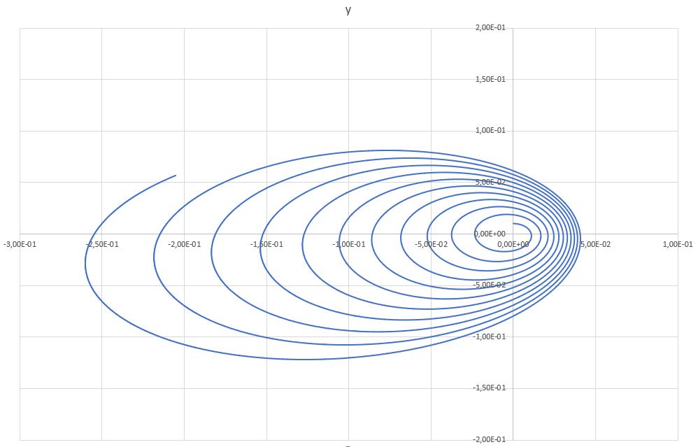
Naively, I thought, that by making the timestep small enough this giveswould give good results. But I observed, that this method is completely bad, because the total energy tends to increase ant what I get is not what I expect:
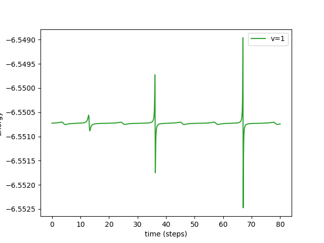
What method for integrating such problem is the standard? My idea is obviously complete garbage because it is numericallythe numerically most unstable. When I calculate the total energy it is not constant at all, even. Even when I make the timestep incredible small, I get totally dissatisfying results.
EDIT: In the meanwhile I read the comment of Daniel Shapero and had a look on his website: https://shapero.xyz/posts/symplectic-integrators/
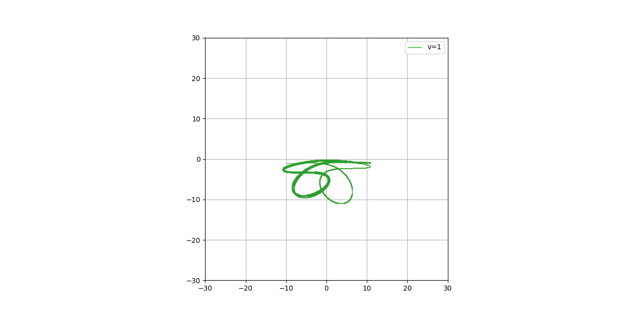
I did a run of pythonPython code using what is referred to as "semi_explicit_euler" for a problem with two fixed masses and one charge coming from the left:
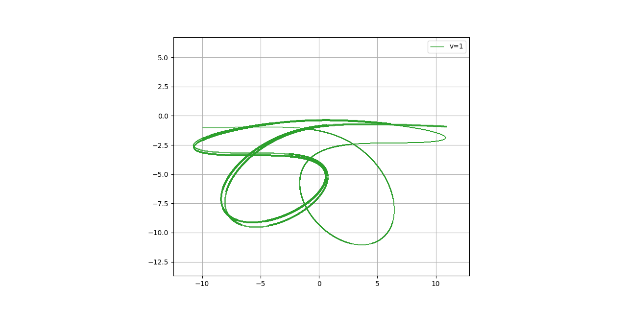
The result is as follows:
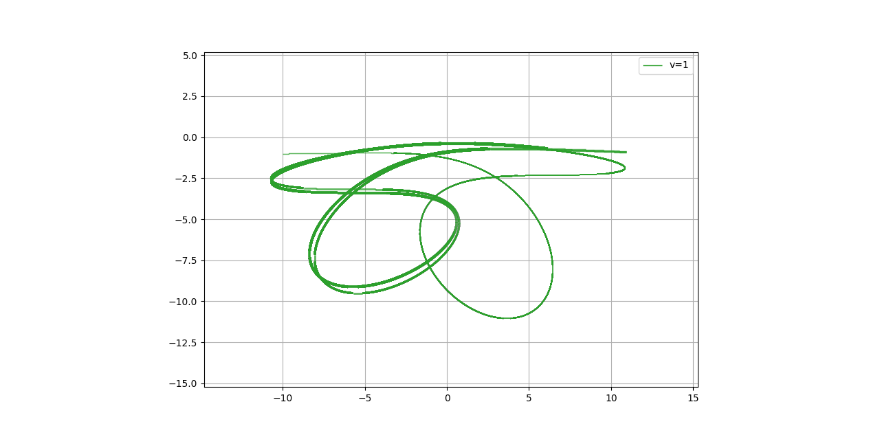
You see that the moving mass stops at the right and gets back. But shouldn't the way back be the same as the way as to the point where it stops? MotionThe motion must be symmetric to time reversal. Interestingly this "discrepancy" is stable and can not be made smaller by increasing the number of steps. The same picture is obtained when the number of steps is only 25% of that:
import numpy as np
from numpy import pi as π
import tqdm
import matplotlib.pyplot as plt
from matplotlib.collections import LineCollection


q_0 = np.array([-10.0, -1])
p_0 = np.array([1.0, 0])
p_1 = np.array([3.0, 0])
p_2 = np.array([5.0, 0])

r1 = np.array([0, 5])
r2 = np.array([0, -5])


final_time = 80.0
num_steps = 2000000*4
dt = final_time / num_steps

def gravitational_force(q, r1, r2):

    return -4 * π ** 2 * (q-r1) / np.sqrt(np.dot((q-r1), (q-r1))) ** 3  -4 * π ** 2 * (q-r2) / np.sqrt(np.dot((q-r2), (q-r2))) ** 3
    #return  -4 * π ** 2 * (q-r2) / np.sqrt(np.dot((q-r2), (q-r2))) ** 3


def semi_explicit_euler(q, p, dt, num_steps, r1, r2, force, progressbar=True):
    qs = np.zeros((num_steps + 1,) + q.shape)
    ps = np.zeros((num_steps + 1,) + p.shape)

    qs[0] = q
    ps[0] = p

    iterator = tqdm.trange(num_steps) if progressbar else range(num_steps)
    for t in iterator:
        qs[t + 1] = qs[t] + dt * ps[t]
        ps[t + 1] = ps[t] + dt * force(qs[t + 1], r1, r2)

    return qs, ps


def plot_trajectory(q, start_width=1.0, end_width=3.0, **kwargs):
    points = q.reshape(-1, 1, 2)
    segments = np.concatenate([points[:-1], points[1:]], axis=1)
    widths = np.linspace(start_width, end_width, len(points))
    return LineCollection(segments, linewidths=widths, **kwargs)


def energies(qs, ps, r1, r2):
    kinetic = 0.5 * np.sum(ps ** 2, axis=1)
    potential = 0
    potential = -4 * π ** 2 / np.sqrt(np.sum((qs-r1) ** 2, axis=1))
    potential = potential - 4 * π ** 2 / np.sqrt(np.sum((qs-r2) ** 2, axis=1))
    return kinetic + potential


q_se0, p_se0 = semi_explicit_euler(q_0, p_0, dt, num_steps, r1, r2, gravitational_force)
#q_se1, p_se1 = semi_explicit_euler(q_0, p_1, dt, num_steps, r1, r2, gravitational_force)
#q_se2, p_se2 = semi_explicit_euler(q_0, p_2, dt, num_steps, r1, r2, gravitational_force)


fig, ax = plt.subplots()
ax.set_aspect("equal")
ax.set_xlim((-30, +30))
ax.set_ylim((-30, +30))
#ax.get_xaxis().set_visible(False)
#ax.get_yaxis().set_visible(False)
ax.grid(True)

ax.add_collection(plot_trajectory(q_se0, color="tab:green", label="v=1"))
#ax.add_collection(plot_trajectory(q_se1, color="tab:blue", label="v=3"))
#ax.add_collection(plot_trajectory(q_se2, color="tab:red", label="v=5"))
ax.legend(loc="upper right")


fig, ax = plt.subplots()
ts = np.linspace(0.0, final_time, num_steps + 1)
ax.plot(ts, energies(q_se0, p_se0, r1, r2), color="tab:green", label="v=1")
#ax.plot(ts, energies(q_se1, p_se1, r1, r2), color="tab:blue",  label="v=3")
#ax.plot(ts, energies(q_se2, p_se2, r1, r2), color="tab:red",   label="v=5")
ax.set_xlabel("time (steps)")
ax.set_ylabel("Energy")
ax.legend()

plt.show()
EDIT: thisThis second question has been solved: The mass doesn't stop, as pointed out in a comment below.
