added 17 characters in body
Source Link
Anton Menshov
  • 8.7k
  • 7
  • 41
  • 94

I am trying to simulate a hyperbolic PDE with some control given by the following:

$u_t(x, t) = u_x(x, t) + \theta(x) u(0, t)$$$u_t(x, t) = u_x(x, t) + \theta(x) u(0, t)$$

with boundary conditions:

$u(1, t) = U(t) = \int_0^1 k(1-y) u(y, t)dy$$$u(1, t) = U(t) = \int_0^1 k(1-y) u(y, t)dy$$

We use the finite difference scheme with initial condition $u(x, 0) = c$ with $c> 0$$c > 0$. i$i$ is discretization in time and j$j$ is in space.

$\frac{u_j^{i+1} - u_j^{i}}{dt} = \frac{u_{j+1}^i - u_{j}^i}{dx} + \theta(x) u_0^i$$$\frac{u_j^{i+1} - u_j^{i}}{dt} = \frac{u_{j+1}^i - u_{j}^i}{dx} + \theta(x) u_0^i$$

Solving yields:

$u_j^{i+1} = u_j^i + dt*(\frac{u_{j+1}^i - u_{j}^i}{dx} + \theta(x) u_0^i)$$$u_j^{i+1} = u_j^i + dt*(\frac{u_{j+1}^i - u_{j}^i}{dx} + \theta(x) u_0^i)$$

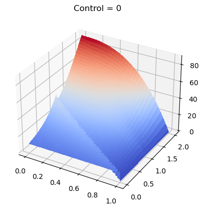
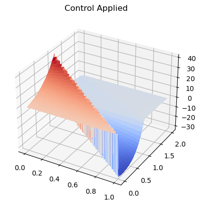
I directly implementimplemented this intoin a Python script and the control seems to work quite well, but I get this very odd looking-looking distribution at the start due to the finite difference scheme. This occurs when I set the control to 0 as well.   

Control = 0   

Control Applied

I believe it is due to the fact the way the initial condition interacts with the time-difference scheme. Is this expected behavior? If not, where is the mistake I am making?

# Simulate PDE to show that this kernel works
T = 2
dt = 0.01
nt = int(round(T/dt))
dx = 0.01
nx = 101
X = np.linspace(0, 1, nx)

u = np.zeros((nt, nx))
c = 10

# Solve for control
def solveControl(kappa, u):
    result = 0
    for i in range(0, nx):
        result += (kappa[nx-i-1]*u[i])*dx
    return result

# Set intial condition
for i in range(nx):
    u[0][i] = c

for i in range(1, nt):
    u[i][-1] = solveControl(kappa, u[i-1])
    for j in range(0, nx-1):
        u[i][j] = u[i-1][j] + dt*((u[i-1][j+1] - u[i-1][j])/dx + theta[j]*u[i-1][0])
I am trying to simulate a hyperbolic PDE with some control given by the following:

$u_t(x, t) = u_x(x, t) + \theta(x) u(0, t)$

with boundary conditions:

$u(1, t) = U(t) = \int_0^1 k(1-y) u(y, t)dy$

We use the finite difference scheme with initial condition $u(x, 0) = c$ with $c> 0$. i is discretization in time and j is in space.

$\frac{u_j^{i+1} - u_j^{i}}{dt} = \frac{u_{j+1}^i - u_{j}^i}{dx} + \theta(x) u_0^i$

Solving yields:

$u_j^{i+1} = u_j^i + dt*(\frac{u_{j+1}^i - u_{j}^i}{dx} + \theta(x) u_0^i)$

I directly implement this into a Python script and the control seems to work quite well, but I get this very odd looking distribution at the start due to the finite difference scheme. This occurs when I set the control to 0 as well.  Control = 0  Control Applied

I believe it is due to the fact the way the initial condition interacts with the time-difference scheme. Is this expected behavior? If not, where is the mistake I am making?

# Simulate PDE to show that this kernel works
T = 2
dt = 0.01
nt = int(round(T/dt))
dx = 0.01
nx = 101
X = np.linspace(0, 1, nx)

u = np.zeros((nt, nx))
c = 10

# Solve for control
def solveControl(kappa, u):
    result = 0
    for i in range(0, nx):
        result += (kappa[nx-i-1]*u[i])*dx
    return result

# Set intial condition
for i in range(nx):
    u[0][i] = c

for i in range(1, nt):
    u[i][-1] = solveControl(kappa, u[i-1])
    for j in range(0, nx-1):
        u[i][j] = u[i-1][j] + dt*((u[i-1][j+1] - u[i-1][j])/dx + theta[j]*u[i-1][0])
I am trying to simulate a hyperbolic PDE with some control given by the following:

$$u_t(x, t) = u_x(x, t) + \theta(x) u(0, t)$$

with boundary conditions:

$$u(1, t) = U(t) = \int_0^1 k(1-y) u(y, t)dy$$

We use the finite difference scheme with initial condition $u(x, 0) = c$ with $c > 0$. $i$ is discretization in time and $j$ is in space.

$$\frac{u_j^{i+1} - u_j^{i}}{dt} = \frac{u_{j+1}^i - u_{j}^i}{dx} + \theta(x) u_0^i$$

Solving yields:

$$u_j^{i+1} = u_j^i + dt*(\frac{u_{j+1}^i - u_{j}^i}{dx} + \theta(x) u_0^i)$$

I directly implemented this in a Python script and the control seems to work quite well, but I get this very odd-looking distribution at the start due to the finite difference scheme. This occurs when I set the control to 0 as well. 

Control = 0 

Control Applied

I believe it is due to the fact the way the initial condition interacts with the time-difference scheme. Is this expected behavior? If not, where is the mistake I am making?

# Simulate PDE to show that this kernel works
T = 2
dt = 0.01
nt = int(round(T/dt))
dx = 0.01
nx = 101
X = np.linspace(0, 1, nx)

u = np.zeros((nt, nx))
c = 10

# Solve for control
def solveControl(kappa, u):
    result = 0
    for i in range(0, nx):
        result += (kappa[nx-i-1]*u[i])*dx
    return result

# Set intial condition
for i in range(nx):
    u[0][i] = c

for i in range(1, nt):
    u[i][-1] = solveControl(kappa, u[i-1])
    for j in range(0, nx-1):
        u[i][j] = u[i-1][j] + dt*((u[i-1][j+1] - u[i-1][j])/dx + theta[j]*u[i-1][0])
edited title
Link

Odd Behavior in Simulating First Order Hyperbolic PDE with Finite Difference Scheme

Source Link

Odd Behavior in Simulating First Order Hyperbolic PDE

I am trying to simulate a hyperbolic PDE with some control given by the following:

$u_t(x, t) = u_x(x, t) + \theta(x) u(0, t)$

with boundary conditions:

$u(1, t) = U(t) = \int_0^1 k(1-y) u(y, t)dy$

We use the finite difference scheme with initial condition $u(x, 0) = c$ with $c> 0$. i is discretization in time and j is in space.

$\frac{u_j^{i+1} - u_j^{i}}{dt} = \frac{u_{j+1}^i - u_{j}^i}{dx} + \theta(x) u_0^i$

Solving yields:

$u_j^{i+1} = u_j^i + dt*(\frac{u_{j+1}^i - u_{j}^i}{dx} + \theta(x) u_0^i)$

I directly implement this into a Python script and the control seems to work quite well, but I get this very odd looking distribution at the start due to the finite difference scheme. This occurs when I set the control to 0 as well. Control = 0 Control Applied

I believe it is due to the fact the way the initial condition interacts with the time-difference scheme. Is this expected behavior? If not, where is the mistake I am making?

# Simulate PDE to show that this kernel works
T = 2
dt = 0.01
nt = int(round(T/dt))
dx = 0.01
nx = 101
X = np.linspace(0, 1, nx)

u = np.zeros((nt, nx))
c = 10

# Solve for control
def solveControl(kappa, u):
    result = 0
    for i in range(0, nx):
        result += (kappa[nx-i-1]*u[i])*dx
    return result

# Set intial condition
for i in range(nx):
    u[0][i] = c

for i in range(1, nt):
    u[i][-1] = solveControl(kappa, u[i-1])
    for j in range(0, nx-1):
        u[i][j] = u[i-1][j] + dt*((u[i-1][j+1] - u[i-1][j])/dx + theta[j]*u[i-1][0])