edited body
Source Link
Royi
  • 563
  • 3
  • 16

I implemented the algorithm in Julia.
The motivation is being able to control better the memory allocations and hence get faster results.

The formulation I used is:

$$\begin{align} \arg \min_{\boldsymbol{x}} \quad & \frac{1}{2} \boldsymbol{x}^{T} \boldsymbol{L} \boldsymbol{x} \\ \text{subject to} \quad & \begin{aligned} {x}_{i} & = {d}_{i} \; \forall i \in \mathcal{V} \\ \end{aligned} \end{align}$$

Where $\mathcal{V}$ is the set of pixel indices which have a reference value.

The trick with the Permutation Matrix allows to order the pixels:

$$ \begin{bmatrix} \boldsymbol{x}_{\mathcal{U}} \\ \boldsymbol{x}_{\mathcal{V}} \end{bmatrix} = \boldsymbol{P} \boldsymbol{x} $$

Since for any Permutation Matrix $ \boldsymbol{P} \boldsymbol{P}^{T} = \boldsymbol{P}^{T} \boldsymbol{P} = \boldsymbol{I} $ then:

$$ \boldsymbol{x}^{T} \boldsymbol{L} \boldsymbol{x} = \boldsymbol{x}^{T} \boldsymbol{P}^{T} \left( \boldsymbol{P} \boldsymbol{L} \boldsymbol{P}^{T} \right) \boldsymbol{P} \boldsymbol{x} = \begin{bmatrix} \boldsymbol{x}_{\mathcal{U}} & \boldsymbol{x}_{\mathcal{V}} \end{bmatrix} \begin{bmatrix} \boldsymbol{L}_{\mathcal{U}} & \boldsymbol{R} \\ \boldsymbol{R} & \boldsymbol{L}_{\mathcal{V}} \end{bmatrix} \begin{bmatrix} \boldsymbol{x}_{\mathcal{U}} \\ \boldsymbol{x}_{\mathcal{V}} \end{bmatrix} $$

Since the permutation matrix means no interaction between pixels (As opposed to equality with general matrix) then one can choose the subset, which interacts with $\boldsymbol{x}_{\mathcal{U}}$, to solve which becomes:

$$\begin{align} \arg \min_{\boldsymbol{x}_{\mathcal{U}}} \quad & \frac{1}{2} \boldsymbol{x}_{\mathcal{U}}^{T} \boldsymbol{L}_{\mathcal{U}} \boldsymbol{x}_{\mathcal{U}} + \frac{1}{2} \boldsymbol{x}_{\mathcal{v}}^{T} \boldsymbol{R} \boldsymbol{x}_{\mathcal{U}} \\ \text{subject to} \quad & \begin{aligned} {x}_{i} & = {d}_{i} \; \forall i \in \mathcal{V} \\ \end{aligned} \end{align}$$

Where $ \boldsymbol{x}_{\mathcal{v}} = \boldsymbol{d} $.
Hence the problem becomes constraint free:

$$ \arg \min_{\boldsymbol{x}_{\mathcal{U}}} \frac{1}{2} \boldsymbol{x}_{\mathcal{U}}^{T} \boldsymbol{L}_{\mathcal{U}} \boldsymbol{x}_{\mathcal{U}} + \frac{1}{2} \boldsymbol{x}_{\mathcal{v}}^{T} \boldsymbol{R} \boldsymbol{x}_{\mathcal{U}} $$

This is a strictly convex problem and the gradient vanishes at:

$$ \boldsymbol{L}_{\mathcal{U}} \hat{\boldsymbol{x}}_{\mathcal{U}} = - \boldsymbol{R} \boldsymbol{x}_{\mathcal{U}} $$$$ \boldsymbol{L}_{\mathcal{U}} \hat{\boldsymbol{x}}_{\mathcal{U}} = - \boldsymbol{R} \boldsymbol{x}_{\mathcal{V}} $$

Which can be solved either directly or using Conjugate Gradient.
The direct solver should take advantage of the fast the matrix is Positive Definite. Since the same matrix is used for 2 image channels, it is better to apply the symbolic factorization once.

The Graph Laplacian Matrix, $\boldsymbol{L} = \boldsymbol{D} - \boldsymbol{W}$, is the result of generating the Affinity / Similarity / Adjacency Matrix and the Degree Matrix.

The weights are calculated by:

$$ {W}_{i, j} \propto \exp\left(- \beta \left| I \left( i \right) - I \left( j \right) \right| \right ) + \epsilon $$

One could choose many more options for affinity / similarity measure.
The added $\epsilon$ assists with numerical difficulties.

The weights should also be normalized.
One could normalize the affinity matrix such that each row has a sum of one as suggested in the question.
The code actually normalizes the distances between the pixels into the range $\left[ 0, 1 \right]$ and then applies the affinity transformation as written above.

I implemented a generalized function to build the weights matrix $\boldsymbol{W}$. It basically loops over the pixels and applies a user defined function which has the input of the 2 values, the indices and the neighborhood shift indices.
This way I could try affinity of 3x3 yet it seems that 4 Connectivity gets better results.
Pay attention not to calculate the self weight (Pixel to itself).

enter image description here

enter image description here

enter image description here

enter image description here

Remarks:

  • The derivation of the objectives follows the solution by @codehippo.
    I rewrote it in a manner clearer to me.
  • The objective is similar to Normal Cuts objective in Graphs.
  • The derivation is equivalent to my Wiki post in case the affinity matrix is indeed normalized to have rows of sum 1. Then the same trick to avoid the equality can be employed.
  • Using Preconditioned CG will be much faster for larger cases.

The code is available on my StackExchange Computational Science GitHub Repository (Look at the ComputationalScience\Q11387 folder).
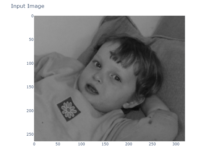
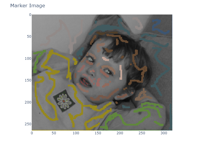
I implemented the algorithm in Julia.
The motivation is being able to control better the memory allocations and hence get faster results.

The formulation I used is:

$$\begin{align} \arg \min_{\boldsymbol{x}} \quad & \frac{1}{2} \boldsymbol{x}^{T} \boldsymbol{L} \boldsymbol{x} \\ \text{subject to} \quad & \begin{aligned} {x}_{i} & = {d}_{i} \; \forall i \in \mathcal{V} \\ \end{aligned} \end{align}$$

Where $\mathcal{V}$ is the set of pixel indices which have a reference value.

The trick with the Permutation Matrix allows to order the pixels:

$$ \begin{bmatrix} \boldsymbol{x}_{\mathcal{U}} \\ \boldsymbol{x}_{\mathcal{V}} \end{bmatrix} = \boldsymbol{P} \boldsymbol{x} $$

Since for any Permutation Matrix $ \boldsymbol{P} \boldsymbol{P}^{T} = \boldsymbol{P}^{T} \boldsymbol{P} = \boldsymbol{I} $ then:

$$ \boldsymbol{x}^{T} \boldsymbol{L} \boldsymbol{x} = \boldsymbol{x}^{T} \boldsymbol{P}^{T} \left( \boldsymbol{P} \boldsymbol{L} \boldsymbol{P}^{T} \right) \boldsymbol{P} \boldsymbol{x} = \begin{bmatrix} \boldsymbol{x}_{\mathcal{U}} & \boldsymbol{x}_{\mathcal{V}} \end{bmatrix} \begin{bmatrix} \boldsymbol{L}_{\mathcal{U}} & \boldsymbol{R} \\ \boldsymbol{R} & \boldsymbol{L}_{\mathcal{V}} \end{bmatrix} \begin{bmatrix} \boldsymbol{x}_{\mathcal{U}} \\ \boldsymbol{x}_{\mathcal{V}} \end{bmatrix} $$

Since the permutation matrix means no interaction between pixels (As opposed to equality with general matrix) then one can choose the subset, which interacts with $\boldsymbol{x}_{\mathcal{U}}$, to solve which becomes:

$$\begin{align} \arg \min_{\boldsymbol{x}_{\mathcal{U}}} \quad & \frac{1}{2} \boldsymbol{x}_{\mathcal{U}}^{T} \boldsymbol{L}_{\mathcal{U}} \boldsymbol{x}_{\mathcal{U}} + \frac{1}{2} \boldsymbol{x}_{\mathcal{v}}^{T} \boldsymbol{R} \boldsymbol{x}_{\mathcal{U}} \\ \text{subject to} \quad & \begin{aligned} {x}_{i} & = {d}_{i} \; \forall i \in \mathcal{V} \\ \end{aligned} \end{align}$$

Where $ \boldsymbol{x}_{\mathcal{v}} = \boldsymbol{d} $.
Hence the problem becomes constraint free:

$$ \arg \min_{\boldsymbol{x}_{\mathcal{U}}} \frac{1}{2} \boldsymbol{x}_{\mathcal{U}}^{T} \boldsymbol{L}_{\mathcal{U}} \boldsymbol{x}_{\mathcal{U}} + \frac{1}{2} \boldsymbol{x}_{\mathcal{v}}^{T} \boldsymbol{R} \boldsymbol{x}_{\mathcal{U}} $$

This is a strictly convex problem and the gradient vanishes at:

$$ \boldsymbol{L}_{\mathcal{U}} \hat{\boldsymbol{x}}_{\mathcal{U}} = - \boldsymbol{R} \boldsymbol{x}_{\mathcal{U}} $$

Which can be solved either directly or using Conjugate Gradient.
The direct solver should take advantage of the fast the matrix is Positive Definite. Since the same matrix is used for 2 image channels, it is better to apply the symbolic factorization once.

The Graph Laplacian Matrix, $\boldsymbol{L} = \boldsymbol{D} - \boldsymbol{W}$, is the result of generating the Affinity / Similarity / Adjacency Matrix and the Degree Matrix.

The weights are calculated by:

$$ {W}_{i, j} \propto \exp\left(- \beta \left| I \left( i \right) - I \left( j \right) \right| \right ) + \epsilon $$

One could choose many more options for affinity / similarity measure.
The added $\epsilon$ assists with numerical difficulties.

The weights should also be normalized.
One could normalize the affinity matrix such that each row has a sum of one as suggested in the question.
The code actually normalizes the distances between the pixels into the range $\left[ 0, 1 \right]$ and then applies the affinity transformation as written above.

I implemented a generalized function to build the weights matrix $\boldsymbol{W}$. It basically loops over the pixels and applies a user defined function which has the input of the 2 values, the indices and the neighborhood shift indices.
This way I could try affinity of 3x3 yet it seems that 4 Connectivity gets better results.
Pay attention not to calculate the self weight (Pixel to itself).

enter image description here

enter image description here

enter image description here

enter image description here

Remarks:

  • The derivation of the objectives follows the solution by @codehippo.
    I rewrote it in a manner clearer to me.
  • The objective is similar to Normal Cuts objective in Graphs.
  • The derivation is equivalent to my Wiki post in case the affinity matrix is indeed normalized to have rows of sum 1. Then the same trick to avoid the equality can be employed.
  • Using Preconditioned CG will be much faster for larger cases.

The code is available on my StackExchange Computational Science GitHub Repository (Look at the ComputationalScience\Q11387 folder).
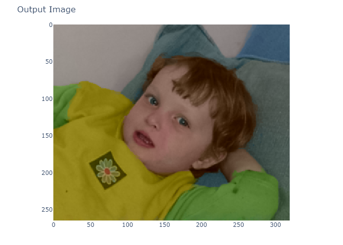
I implemented the algorithm in Julia.
The motivation is being able to control better the memory allocations and hence get faster results.

The formulation I used is:

$$\begin{align} \arg \min_{\boldsymbol{x}} \quad & \frac{1}{2} \boldsymbol{x}^{T} \boldsymbol{L} \boldsymbol{x} \\ \text{subject to} \quad & \begin{aligned} {x}_{i} & = {d}_{i} \; \forall i \in \mathcal{V} \\ \end{aligned} \end{align}$$

Where $\mathcal{V}$ is the set of pixel indices which have a reference value.

The trick with the Permutation Matrix allows to order the pixels:

$$ \begin{bmatrix} \boldsymbol{x}_{\mathcal{U}} \\ \boldsymbol{x}_{\mathcal{V}} \end{bmatrix} = \boldsymbol{P} \boldsymbol{x} $$

Since for any Permutation Matrix $ \boldsymbol{P} \boldsymbol{P}^{T} = \boldsymbol{P}^{T} \boldsymbol{P} = \boldsymbol{I} $ then:

$$ \boldsymbol{x}^{T} \boldsymbol{L} \boldsymbol{x} = \boldsymbol{x}^{T} \boldsymbol{P}^{T} \left( \boldsymbol{P} \boldsymbol{L} \boldsymbol{P}^{T} \right) \boldsymbol{P} \boldsymbol{x} = \begin{bmatrix} \boldsymbol{x}_{\mathcal{U}} & \boldsymbol{x}_{\mathcal{V}} \end{bmatrix} \begin{bmatrix} \boldsymbol{L}_{\mathcal{U}} & \boldsymbol{R} \\ \boldsymbol{R} & \boldsymbol{L}_{\mathcal{V}} \end{bmatrix} \begin{bmatrix} \boldsymbol{x}_{\mathcal{U}} \\ \boldsymbol{x}_{\mathcal{V}} \end{bmatrix} $$

Since the permutation matrix means no interaction between pixels (As opposed to equality with general matrix) then one can choose the subset, which interacts with $\boldsymbol{x}_{\mathcal{U}}$, to solve which becomes:

$$\begin{align} \arg \min_{\boldsymbol{x}_{\mathcal{U}}} \quad & \frac{1}{2} \boldsymbol{x}_{\mathcal{U}}^{T} \boldsymbol{L}_{\mathcal{U}} \boldsymbol{x}_{\mathcal{U}} + \frac{1}{2} \boldsymbol{x}_{\mathcal{v}}^{T} \boldsymbol{R} \boldsymbol{x}_{\mathcal{U}} \\ \text{subject to} \quad & \begin{aligned} {x}_{i} & = {d}_{i} \; \forall i \in \mathcal{V} \\ \end{aligned} \end{align}$$

Where $ \boldsymbol{x}_{\mathcal{v}} = \boldsymbol{d} $.
Hence the problem becomes constraint free:

$$ \arg \min_{\boldsymbol{x}_{\mathcal{U}}} \frac{1}{2} \boldsymbol{x}_{\mathcal{U}}^{T} \boldsymbol{L}_{\mathcal{U}} \boldsymbol{x}_{\mathcal{U}} + \frac{1}{2} \boldsymbol{x}_{\mathcal{v}}^{T} \boldsymbol{R} \boldsymbol{x}_{\mathcal{U}} $$

This is a strictly convex problem and the gradient vanishes at:

$$ \boldsymbol{L}_{\mathcal{U}} \hat{\boldsymbol{x}}_{\mathcal{U}} = - \boldsymbol{R} \boldsymbol{x}_{\mathcal{V}} $$

Which can be solved either directly or using Conjugate Gradient.
The direct solver should take advantage of the fast the matrix is Positive Definite. Since the same matrix is used for 2 image channels, it is better to apply the symbolic factorization once.

The Graph Laplacian Matrix, $\boldsymbol{L} = \boldsymbol{D} - \boldsymbol{W}$, is the result of generating the Affinity / Similarity / Adjacency Matrix and the Degree Matrix.

The weights are calculated by:

$$ {W}_{i, j} \propto \exp\left(- \beta \left| I \left( i \right) - I \left( j \right) \right| \right ) + \epsilon $$

One could choose many more options for affinity / similarity measure.
The added $\epsilon$ assists with numerical difficulties.

The weights should also be normalized.
One could normalize the affinity matrix such that each row has a sum of one as suggested in the question.
The code actually normalizes the distances between the pixels into the range $\left[ 0, 1 \right]$ and then applies the affinity transformation as written above.

I implemented a generalized function to build the weights matrix $\boldsymbol{W}$. It basically loops over the pixels and applies a user defined function which has the input of the 2 values, the indices and the neighborhood shift indices.
This way I could try affinity of 3x3 yet it seems that 4 Connectivity gets better results.
Pay attention not to calculate the self weight (Pixel to itself).

enter image description here

enter image description here

enter image description here

enter image description here

Remarks:

  • The derivation of the objectives follows the solution by @codehippo.
    I rewrote it in a manner clearer to me.
  • The objective is similar to Normal Cuts objective in Graphs.
  • The derivation is equivalent to my Wiki post in case the affinity matrix is indeed normalized to have rows of sum 1. Then the same trick to avoid the equality can be employed.
  • Using Preconditioned CG will be much faster for larger cases.

The code is available on my StackExchange Computational Science GitHub Repository (Look at the ComputationalScience\Q11387 folder).
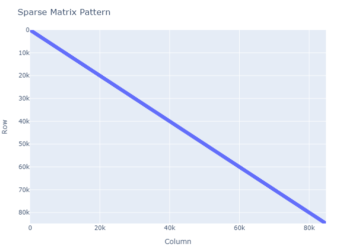
added 246 characters in body
Source Link
Royi
  • 563
  • 3
  • 16

I implemented the algorithm in Julia.
The motivation is being able to control better the memory allocations and hence get faster results.

The formulation I used is:

$$\begin{align} \arg \min_{\boldsymbol{x}} \quad & \frac{1}{2} \boldsymbol{x}^{T} \boldsymbol{L} \boldsymbol{x} \\ \text{subject to} \quad & \begin{aligned} {x}_{i} & = {d}_{i} \; \forall i \in \mathcal{V} \\ \end{aligned} \end{align}$$

Where $\mathcal{V}$ is the set of pixel indices which have a reference value.

The trick with the Permutation Matrix allows to order the pixels:

$$ \begin{bmatrix} \boldsymbol{x}_{\mathcal{U}} \\ \boldsymbol{x}_{\mathcal{V}} \end{bmatrix} = \boldsymbol{P} \boldsymbol{x} $$

Since for any Permutation Matrix $ \boldsymbol{P} \boldsymbol{P}^{T} = \boldsymbol{P}^{T} \boldsymbol{P} = \boldsymbol{I} $ then:

$$ \boldsymbol{x}^{T} \boldsymbol{L} \boldsymbol{x} = \boldsymbol{x}^{T} \boldsymbol{P}^{T} \left( \boldsymbol{P} \boldsymbol{L} \boldsymbol{P}^{T} \right) \boldsymbol{P} \boldsymbol{x} = \begin{bmatrix} \boldsymbol{x}_{\mathcal{U}} & \boldsymbol{x}_{\mathcal{V}} \end{bmatrix} \begin{bmatrix} \boldsymbol{L}_{\mathcal{U}} & \boldsymbol{R} \\ \boldsymbol{R} & \boldsymbol{L}_{\mathcal{V}} \end{bmatrix} \begin{bmatrix} \boldsymbol{x}_{\mathcal{U}} \\ \boldsymbol{x}_{\mathcal{V}} \end{bmatrix} $$

Since the permutation matrix means no interaction between pixels (As opposed to equality with general matrix) then one can choose the subset, which interacts with $\boldsymbol{x}_{\mathcal{U}}$, to solve which becomes:

$$\begin{align} \arg \min_{\boldsymbol{x}_{\mathcal{U}}} \quad & \frac{1}{2} \boldsymbol{x}_{\mathcal{U}}^{T} \boldsymbol{L}_{\mathcal{U}} \boldsymbol{x}_{\mathcal{U}} + \frac{1}{2} \boldsymbol{x}_{\mathcal{v}}^{T} \boldsymbol{R} \boldsymbol{x}_{\mathcal{U}} \\ \text{subject to} \quad & \begin{aligned} {x}_{i} & = {d}_{i} \; \forall i \in \mathcal{V} \\ \end{aligned} \end{align}$$

Where $ \boldsymbol{x}_{\mathcal{v}} = \boldsymbol{d} $.
Hence the problem becomes constraint free:

$$ \arg \min_{\boldsymbol{x}_{\mathcal{U}}} \frac{1}{2} \boldsymbol{x}_{\mathcal{U}}^{T} \boldsymbol{L}_{\mathcal{U}} \boldsymbol{x}_{\mathcal{U}} + \frac{1}{2} \boldsymbol{x}_{\mathcal{v}}^{T} \boldsymbol{R} \boldsymbol{x}_{\mathcal{U}} $$

This is a strictly convex problem and the gradient vanishes at:

$$ \boldsymbol{L}_{\mathcal{U}} \hat{\boldsymbol{x}}_{\mathcal{U}} = - \boldsymbol{R} \boldsymbol{x}_{\mathcal{U}} $$

Which can be solved either directly or using Conjugate Gradient.
The direct solver should take advantage of the fast the matrix is Positive Definite. Since the same matrix is used for 2 image channels, it is better to apply the symbolic factorization once.

The Graph Laplacian Matrix, $\boldsymbol{L} = \boldsymbol{D} - \boldsymbol{W}$, is the result of generating the Affinity / Similarity / Adjacency Matrix and the Degree Matrix.

The weights are calculated by:

$$ {W}_{i, j} \propto \exp\left(- \beta \left| I \left( i \right) - I \left( j \right) \right| \right ) + \epsilon $$

One could choose many more options for affinity / similarity measure.
The added $\epsilon$ assists with numerical difficulties.

The weights should also be normalized.
One could normalize the affinity matrix such that each row has a sum of one as suggested in the question.
The code actually normalizes the distances between the pixels into the range $\left[ 0, 1 \right]$ and then applies the affinity transformation as written above.

I implemented a generalized function to build the weights matrix $\boldsymbol{W}$. It basically loops over the pixels and applies a user defined function which has the input of the 2 values, the indices and the neighborhood shift indices.
This way I could try affinity of 3x3 yet it seems that 4 Connectivity gets better results.
Pay attention not to calculate the self weight (Pixel to itself).

enter image description here

enter image description here

enter image description here

enter image description here

Remarks:

  • The derivation of the objectives follows the solution by @codehippo.
    I rewrote it in a manner clearer to me.
  • The objective is similar to Normal Cuts objective in Graphs.
  • The derivation is equivalent to my Wiki post in case the affinity matrix is indeed normalized to have rows of sum 1. Then the same trick to avoid the equality can be employed.
  • Using Preconditioned CG will be much faster for larger cases.

The code is available on my StackExchange Computational Science GitHub Repository (Look at the ComputationalScience\Q11387 folder).

I implemented the algorithm in Julia.
The motivation is being able to control better the memory allocations and hence get faster results.

The formulation I used is:

$$\begin{align} \arg \min_{\boldsymbol{x}} \quad & \frac{1}{2} \boldsymbol{x}^{T} \boldsymbol{L} \boldsymbol{x} \\ \text{subject to} \quad & \begin{aligned} {x}_{i} & = {d}_{i} \; \forall i \in \mathcal{V} \\ \end{aligned} \end{align}$$

Where $\mathcal{V}$ is the set of pixel indices which have a reference value.

The trick with the Permutation Matrix allows to order the pixels:

$$ \begin{bmatrix} \boldsymbol{x}_{\mathcal{U}} \\ \boldsymbol{x}_{\mathcal{V}} \end{bmatrix} = \boldsymbol{P} \boldsymbol{x} $$

Since for any Permutation Matrix $ \boldsymbol{P} \boldsymbol{P}^{T} = \boldsymbol{P}^{T} \boldsymbol{P} = \boldsymbol{I} $ then:

$$ \boldsymbol{x}^{T} \boldsymbol{L} \boldsymbol{x} = \boldsymbol{x}^{T} \boldsymbol{P}^{T} \left( \boldsymbol{P} \boldsymbol{L} \boldsymbol{P}^{T} \right) \boldsymbol{P} \boldsymbol{x} = \begin{bmatrix} \boldsymbol{x}_{\mathcal{U}} & \boldsymbol{x}_{\mathcal{V}} \end{bmatrix} \begin{bmatrix} \boldsymbol{L}_{\mathcal{U}} & \boldsymbol{R} \\ \boldsymbol{R} & \boldsymbol{L}_{\mathcal{V}} \end{bmatrix} \begin{bmatrix} \boldsymbol{x}_{\mathcal{U}} \\ \boldsymbol{x}_{\mathcal{V}} \end{bmatrix} $$

Since the permutation matrix means no interaction between pixels (As opposed to equality with general matrix) then one can choose the subset, which interacts with $\boldsymbol{x}_{\mathcal{U}}$, to solve which becomes:

$$\begin{align} \arg \min_{\boldsymbol{x}_{\mathcal{U}}} \quad & \frac{1}{2} \boldsymbol{x}_{\mathcal{U}}^{T} \boldsymbol{L}_{\mathcal{U}} \boldsymbol{x}_{\mathcal{U}} + \frac{1}{2} \boldsymbol{x}_{\mathcal{v}}^{T} \boldsymbol{R} \boldsymbol{x}_{\mathcal{U}} \\ \text{subject to} \quad & \begin{aligned} {x}_{i} & = {d}_{i} \; \forall i \in \mathcal{V} \\ \end{aligned} \end{align}$$

Where $ \boldsymbol{x}_{\mathcal{v}} = \boldsymbol{d} $.
Hence the problem becomes constraint free:

$$ \arg \min_{\boldsymbol{x}_{\mathcal{U}}} \frac{1}{2} \boldsymbol{x}_{\mathcal{U}}^{T} \boldsymbol{L}_{\mathcal{U}} \boldsymbol{x}_{\mathcal{U}} + \frac{1}{2} \boldsymbol{x}_{\mathcal{v}}^{T} \boldsymbol{R} \boldsymbol{x}_{\mathcal{U}} $$

This is a strictly convex problem and the gradient vanishes at:

$$ \boldsymbol{L}_{\mathcal{U}} \hat{\boldsymbol{x}}_{\mathcal{U}} = - \boldsymbol{R} \boldsymbol{x}_{\mathcal{U}} $$

Which can be solved either directly or using Conjugate Gradient.
The direct solver should take advantage of the fast the matrix is Positive Definite. Since the same matrix is used for 2 image channels, it is better to apply the symbolic factorization once.

The Graph Laplacian Matrix, $\boldsymbol{L} = \boldsymbol{D} - \boldsymbol{W}$, is the result of generating the Affinity / Similarity / Adjacency Matrix and the Degree Matrix.

The weights are calculated by:

$$ {W}_{i, j} \propto \exp\left(- \beta \left| I \left( i \right) - I \left( j \right) \right| \right ) + \epsilon $$

One could choose many more options for affinity / similarity measure.
The added $\epsilon$ assists with numerical difficulties.

The weights should also be normalized.
One could normalize the affinity matrix such that each row has a sum of one as suggested in the question.
The code actually normalizes the distances between the pixels into the range $\left[ 0, 1 \right]$ and then applies the affinity transformation as written above.

I implemented a generalized function to build the weights matrix $\boldsymbol{W}$. It basically loops over the pixels and applies a user defined function which has the input of the 2 values, the indices and the neighborhood shift indices.
This way I could try affinity of 3x3 yet it seems that 4 Connectivity gets better results.
Pay attention not to calculate the self weight (Pixel to itself).

enter image description here

enter image description here

enter image description here

enter image description here

Remarks:

  • The derivation of the objectives follows the solution by @codehippo.
    I rewrote it in a manner clearer to me.
  • The objective is similar to Normal Cuts objective in Graphs.
  • The derivation is equivalent to my Wiki post in case the affinity matrix is indeed normalized to have rows of sum 1. Then the same trick to avoid the equality can be employed.
  • Using Preconditioned CG will be much faster for larger cases.

The code is available on my StackExchange Computational Science GitHub Repository (Look at the ComputationalScience\Q11387 folder).

Source Link
Royi
  • 563
  • 3
  • 16

I implemented the algorithm in Julia.
The motivation is being able to control better the memory allocations and hence get faster results.

The formulation I used is:

$$\begin{align} \arg \min_{\boldsymbol{x}} \quad & \frac{1}{2} \boldsymbol{x}^{T} \boldsymbol{L} \boldsymbol{x} \\ \text{subject to} \quad & \begin{aligned} {x}_{i} & = {d}_{i} \; \forall i \in \mathcal{V} \\ \end{aligned} \end{align}$$

Where $\mathcal{V}$ is the set of pixel indices which have a reference value.

The trick with the Permutation Matrix allows to order the pixels:

$$ \begin{bmatrix} \boldsymbol{x}_{\mathcal{U}} \\ \boldsymbol{x}_{\mathcal{V}} \end{bmatrix} = \boldsymbol{P} \boldsymbol{x} $$

Since for any Permutation Matrix $ \boldsymbol{P} \boldsymbol{P}^{T} = \boldsymbol{P}^{T} \boldsymbol{P} = \boldsymbol{I} $ then:

$$ \boldsymbol{x}^{T} \boldsymbol{L} \boldsymbol{x} = \boldsymbol{x}^{T} \boldsymbol{P}^{T} \left( \boldsymbol{P} \boldsymbol{L} \boldsymbol{P}^{T} \right) \boldsymbol{P} \boldsymbol{x} = \begin{bmatrix} \boldsymbol{x}_{\mathcal{U}} & \boldsymbol{x}_{\mathcal{V}} \end{bmatrix} \begin{bmatrix} \boldsymbol{L}_{\mathcal{U}} & \boldsymbol{R} \\ \boldsymbol{R} & \boldsymbol{L}_{\mathcal{V}} \end{bmatrix} \begin{bmatrix} \boldsymbol{x}_{\mathcal{U}} \\ \boldsymbol{x}_{\mathcal{V}} \end{bmatrix} $$

Since the permutation matrix means no interaction between pixels (As opposed to equality with general matrix) then one can choose the subset, which interacts with $\boldsymbol{x}_{\mathcal{U}}$, to solve which becomes:

$$\begin{align} \arg \min_{\boldsymbol{x}_{\mathcal{U}}} \quad & \frac{1}{2} \boldsymbol{x}_{\mathcal{U}}^{T} \boldsymbol{L}_{\mathcal{U}} \boldsymbol{x}_{\mathcal{U}} + \frac{1}{2} \boldsymbol{x}_{\mathcal{v}}^{T} \boldsymbol{R} \boldsymbol{x}_{\mathcal{U}} \\ \text{subject to} \quad & \begin{aligned} {x}_{i} & = {d}_{i} \; \forall i \in \mathcal{V} \\ \end{aligned} \end{align}$$

Where $ \boldsymbol{x}_{\mathcal{v}} = \boldsymbol{d} $.
Hence the problem becomes constraint free:

$$ \arg \min_{\boldsymbol{x}_{\mathcal{U}}} \frac{1}{2} \boldsymbol{x}_{\mathcal{U}}^{T} \boldsymbol{L}_{\mathcal{U}} \boldsymbol{x}_{\mathcal{U}} + \frac{1}{2} \boldsymbol{x}_{\mathcal{v}}^{T} \boldsymbol{R} \boldsymbol{x}_{\mathcal{U}} $$

This is a strictly convex problem and the gradient vanishes at:

$$ \boldsymbol{L}_{\mathcal{U}} \hat{\boldsymbol{x}}_{\mathcal{U}} = - \boldsymbol{R} \boldsymbol{x}_{\mathcal{U}} $$

Which can be solved either directly or using Conjugate Gradient.
The direct solver should take advantage of the fast the matrix is Positive Definite. Since the same matrix is used for 2 image channels, it is better to apply the symbolic factorization once.

The Graph Laplacian Matrix, $\boldsymbol{L} = \boldsymbol{D} - \boldsymbol{W}$, is the result of generating the Affinity / Similarity / Adjacency Matrix and the Degree Matrix.

The weights are calculated by:

$$ {W}_{i, j} \propto \exp\left(- \beta \left| I \left( i \right) - I \left( j \right) \right| \right ) + \epsilon $$

One could choose many more options for affinity / similarity measure.
The added $\epsilon$ assists with numerical difficulties.

The weights should also be normalized.
One could normalize the affinity matrix such that each row has a sum of one as suggested in the question.
The code actually normalizes the distances between the pixels into the range $\left[ 0, 1 \right]$ and then applies the affinity transformation as written above.

I implemented a generalized function to build the weights matrix $\boldsymbol{W}$. It basically loops over the pixels and applies a user defined function which has the input of the 2 values, the indices and the neighborhood shift indices.
This way I could try affinity of 3x3 yet it seems that 4 Connectivity gets better results.
Pay attention not to calculate the self weight (Pixel to itself).

enter image description here

enter image description here

enter image description here

enter image description here

Remarks:

  • The derivation of the objectives follows the solution by @codehippo.
    I rewrote it in a manner clearer to me.
  • The objective is similar to Normal Cuts objective in Graphs.

The code is available on my StackExchange Computational Science GitHub Repository (Look at the ComputationalScience\Q11387 folder).