replaced http://scicomp.stackexchange.com/ with https://scicomp.stackexchange.com/
Source Link

A few words of warning. This is basic solution you wanted, but you will need to include some sort of boundary condition for a well-posed problem. Also, Crank-Nicolson is not necessarily the best method for the advection equation. It is second order accurate and unconditionally stableunconditionally stable, which is fantastic. However it will generate (as with all centered difference stencils) spurious oscillation if you have very sharp peaked solutions or initial conditions.

A few words of warning. This is basic solution you wanted, but you will need to include some sort of boundary condition for a well-posed problem. Also, Crank-Nicolson is not necessarily the best method for the advection equation. It is second order accurate and unconditionally stable, which is fantastic. However it will generate (as with all centered difference stencils) spurious oscillation if you have very sharp peaked solutions or initial conditions.

A few words of warning. This is basic solution you wanted, but you will need to include some sort of boundary condition for a well-posed problem. Also, Crank-Nicolson is not necessarily the best method for the advection equation. It is second order accurate and unconditionally stable, which is fantastic. However it will generate (as with all centered difference stencils) spurious oscillation if you have very sharp peaked solutions or initial conditions.

Bounty Ended with 100 reputation awarded by CommunityBot
Cleaned up the code a little bit
Source Link
boyfarrell
  • 5.4k
  • 3
  • 35
  • 67
from __future__ import division
from scipy.sparse import spdiags
from scipy.sparse.linalg import spsolve
import numpy as np
 
beta = 0.5
J = 200 # total number of mesh points
z = np.linspace(-10,10,J) # vertices
dz = abs(z[1]-z[0]) # space step
dt = 0.2    # time step
v = 2 * np.ones(len(z)) # velocity field (constant)
r = v / 2 * dt / dz

# initial conditions
gaussian = lambda z, height, position, hwhm: height * np.exp(-np.log(2) * ((z - position)/hwhm)**2)
u_init = gaussian(z, 1, -3,import 2)pylab
    
def make_advection_matrices(z, r):
    """Return matrices A and M for advection equations"""
    lower = -beta * r; centreones = np.ones(len(z)); upper = beta * r
    A = spdiags( [lower[-beta*r, centreones, upper]beta*r], (-1,0,1), len(z), len(z) )
    
    lowerM = spdiags( [(1-beta) * r; centre =r, np.ones(len(z)); upper =, -(1-beta) * r
    M = spdiags( [lower, centre, upper]r], (-1,0,1), len(z), len(z) )
    return A.tocsr(), M.tocsr()

def plot_iteration(z, u, iteration):
    """Plot the solver progress"""
    import pylab
    pylab.plot(z, u, label="Iteration %d" % iteration) 

# Set up basic pylabconstants
beta = 0.savefig5
J = 200 # total number of mesh points
z = np.linspace("%d_solution"-10,10,J) %# iterationvertices
dz = abs(z[1]-z[0]) # space step
dt = 0.2  pylab  # time step
v = 2 * np.claones(len(z)) # velocity field (constant)
r = v / 2 * dt / dz

# Initial conditions (peak function)
gaussian = lambda z, height, position, hwhm: height * np.exp(-np.log(2) * ((z - position)/hwhm)**2)
u_init = gaussian(z, 1, -3, 2)

A, M = make_advection_matrices(z, r)
u = u_init
for i in range(10):
    d = M * u
    u = spsolve(A, M * u)
    plot_iteration(z, u, i)

pylab.legend()
pylab.show()
from __future__ import division
from scipy.sparse import spdiags
from scipy.sparse.linalg import spsolve
import numpy as np
 
beta = 0.5
J = 200 # total number of mesh points
z = np.linspace(-10,10,J) # vertices
dz = abs(z[1]-z[0]) # space step
dt = 0.2    # time step
v = 2 * np.ones(len(z)) # velocity field (constant)
r = v / 2 * dt / dz

# initial conditions
gaussian = lambda z, height, position, hwhm: height * np.exp(-np.log(2) * ((z - position)/hwhm)**2)
u_init = gaussian(z, 1, -3, 2)
    
def make_advection_matrices(z, r):
    """Return matrices A and M for advection equations"""
    lower = -beta * r; centre = np.ones(len(z)); upper = beta * r
    A = spdiags( [lower, centre, upper], (-1,0,1), len(z), len(z) )
    
    lower = (1-beta) * r; centre = np.ones(len(z)); upper = -(1-beta) * r
    M = spdiags( [lower, centre, upper], (-1,0,1), len(z), len(z) )
    return A.tocsr(), M.tocsr()

def plot_iteration(z, u, iteration):
    """Plot the solver progress"""
    import pylab
    pylab.plot(z, u, label="Iteration %d" % iteration)
    pylab.savefig("%d_solution" % iteration)
    pylab.cla()
    
A, M = make_advection_matrices(z, r)
u = u_init
for i in range(10):
    d = M * u
    u = spsolve(A, M * u)
    plot_iteration(z, u, i)
from __future__ import division
from scipy.sparse import spdiags
from scipy.sparse.linalg import spsolve
import numpy as np
import pylab

def make_advection_matrices(z, r):
    """Return matrices A and M for advection equations"""
    ones = np.ones(len(z))
    A = spdiags( [-beta*r, ones, beta*r], (-1,0,1), len(z), len(z) )
    M = spdiags( [(1-beta) * r, ones, -(1-beta) * r], (-1,0,1), len(z), len(z) )
    return A.tocsr(), M.tocsr()

def plot_iteration(z, u, iteration):
    """Plot the solver progress"""
    pylab.plot(z, u, label="Iteration %d" % iteration) 

# Set up basic constants
beta = 0.5
J = 200 # total number of mesh points
z = np.linspace(-10,10,J) # vertices
dz = abs(z[1]-z[0]) # space step
dt = 0.2    # time step
v = 2 * np.ones(len(z)) # velocity field (constant)
r = v / 2 * dt / dz

# Initial conditions (peak function)
gaussian = lambda z, height, position, hwhm: height * np.exp(-np.log(2) * ((z - position)/hwhm)**2)
u_init = gaussian(z, 1, -3, 2)

A, M = make_advection_matrices(z, r)
u = u_init
for i in range(10):
    u = spsolve(A, M * u)
    plot_iteration(z, u, i)

pylab.legend()
pylab.show()
Typo.
Source Link
boyfarrell
  • 5.4k
  • 3
  • 35
  • 67

A few workswords of warning. This is basic solution you wanted, but you will need to include some sort of boundary condition for a well-posed problem. Also, Crank-Nicolson is not necessarily the best method for the advection equation. IfIt is second order accurate and unconditionally stable, which is fantastic. However it will generate (as with all centered difference stencils) spurious oscillation if you have very sharp peaked solutions or initial conditions.

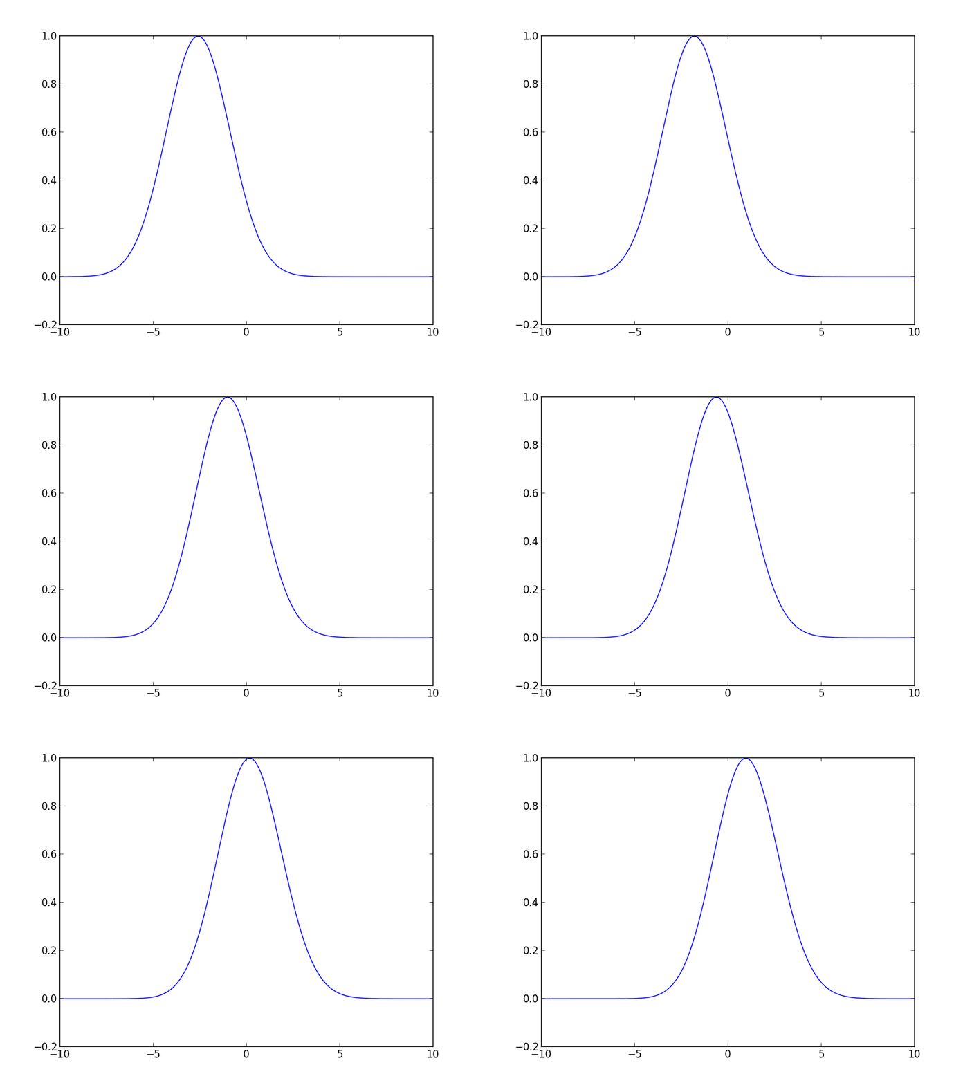
I just spentwrote the last 30 minutes writing thisfollowing code for you in Python. It, it should get you started. The code solves athe advection equation for an initial Gaussian curve advectingmoving to the right with constant velocity.

Gaussian curve advecting to the right at constant velocityGaussian curve moving to the right with constant velocity

A few works of warning. This is basic solution you wanted, but you will need to include some sort of boundary condition for a well-posed problem. Also, Crank-Nicolson is not necessarily the best method for the advection equation. If is second order accurate and unconditionally stable, which is fantastic. However it will generate (as with all centered difference stencils) spurious oscillation if you have very sharp peaked solutions or initial conditions.

I just spent the last 30 minutes writing this in Python. It should get you started. The code solves a Gaussian curve advecting to the right with constant velocity.

Gaussian curve advecting to the right at constant velocity

A few words of warning. This is basic solution you wanted, but you will need to include some sort of boundary condition for a well-posed problem. Also, Crank-Nicolson is not necessarily the best method for the advection equation. It is second order accurate and unconditionally stable, which is fantastic. However it will generate (as with all centered difference stencils) spurious oscillation if you have very sharp peaked solutions or initial conditions.

I wrote the following code for you in Python, it should get you started. The code solves the advection equation for an initial Gaussian curve moving to the right with constant velocity.

Gaussian curve moving to the right with constant velocity

Added some python source code which solves the advection equation with Crank-Nicolson
Source Link
boyfarrell
  • 5.4k
  • 3
  • 35
  • 67
Loading
Source Link
boyfarrell
  • 5.4k
  • 3
  • 35
  • 67
Loading