Using scipy.quad to calculate difficult integral

Question

When evaluating the integral below in python using scipy.quad I get the following warning:

UserWarning: The maximum number of subdivisions (50) has been achieved. If increasing the limit yields no improvement it is advised to analyze the integrand in order to determine the difficulties. If the position of a local difficulty can be determined (singularity, discontinuity) one will probably gain from splitting up the interval and calling the integrator on the subranges. Perhaps a special-purpose integrator should be used.

Furthermore the real integration bounds should be zero to infinity (see below) but when I change the bounds to this my result looks very different from the finite values used in my example below. How should I go about calculating this integral?

I have the following complex integral to compute numerically:

\begin{align} \int_0^{\infty} Re \left( \frac{t_1(s)-it_2(s)}{\sqrt{\zeta^2(s)-1}} \right) \exp(i\omega s/V) \, \mathrm{d}s \end{align}

here $i=\sqrt{-1}$, $t_1$ and $t_2$ are real parametric functions of $s$, $V=\frac{\pi}{2(\pi+2)}$ is a constant, and $\zeta(s)$ is a complex function of $s$. The functions $t_1$, $t_2$, and $\zeta$ are not available in closed form, rather I have computed them numerically. A numpy array containing the sampled function values at various vales of s can be found to download at http://speedy.sh/prG9e/stackexchange.npy. The integrand is problematic because $\zeta(0) = 1$.

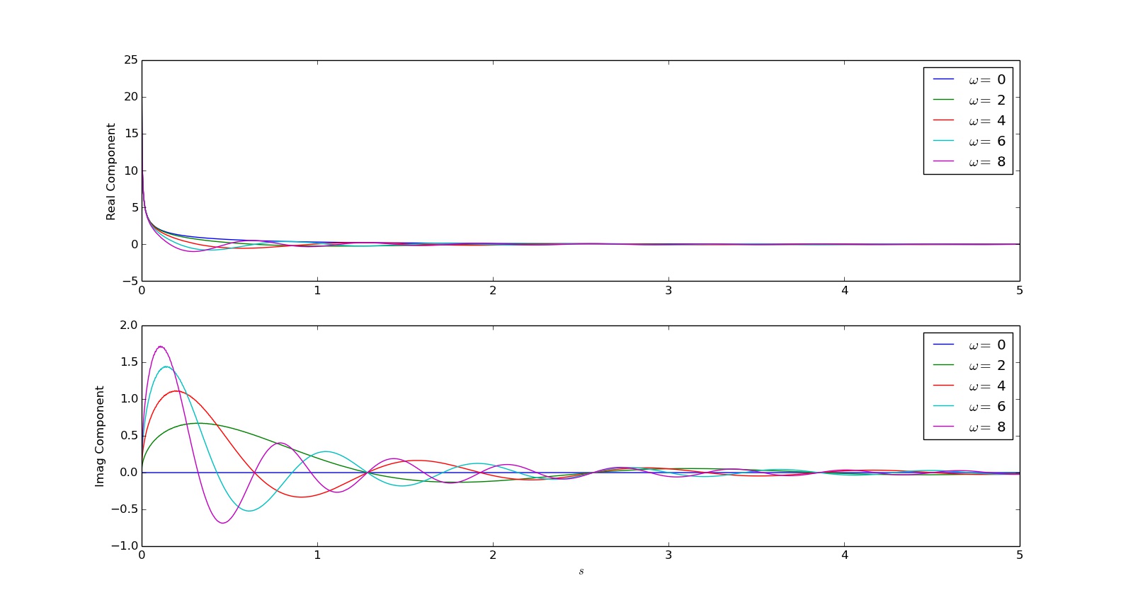
I have plotted the integrands for various values of omega:

The singularity in the real integrand is apparent. My work so far:

import numpy as np
import matplotlib.pyplot as plt
from scipy import integrate

T2 = np.load('stackexchange.npy') #Data: [s, x1, x2, t1, t2]

def pyfunc(z):
    return np.sqrt(z**2-1)

def integrand(s, omega):
    x1 = np.interp(s, T2[:,0], T2[:,1] )
    x2 = np.interp(s, T2[:,0], T2[:,2] )
    t1 = np.interp(s, T2[:,0], T2[:,3] )
    t2 = np.interp(s, T2[:,0], T2[:,4] )
    zeta = x2+x1*1j
    sigma = np.pi/(np.pi+2) 
    V = 1/(2*sigma) 
    return (-t2*np.real(1j/pyfunc(zeta))+t1*np.real(1/pyfunc(zeta)))*np.exp(1j*omega*s/V)


def integral(omega):
    def real_func(x,omega):
        return np.real(integrand(x,omega))
    def imag_func(x,omega):
        return np.imag(integrand(x,omega))
    a = 0.05 #Lower bound
    b = 20.0 #Upper bound
    real_integral = integrate.quad(real_func, a, b, args=(omega))
    imag_integral = integrate.quad(imag_func, a, b, args=(omega))   
    return real_integral[0] + 1j*imag_integral[0]

vintegral = np.vectorize(integral)

omega = np.linspace(-30, 30, 601)
I = integral(omega)

plt.plot(omega, I.real, omega, I.imag)
plt.show()

Edit

I found an analytical representation of the integrand in question, defined below. It still seems that there are some numerical difficulties with it though as NaNs are returned when I try to integrate.

    def pyfunc(z):
        return np.sqrt(z**2-1)  

    def func(theta):
        t1 = 1/np.sqrt(1+np.tan(theta)**2)    
        t2 = -1/np.sqrt(1+1/np.tan(theta)**2)
        return t1, t2


    def integrand(s, omega):
            sigma = np.pi/(np.pi+2) 
            xs = np.exp(-np.pi*s/(2*sigma))
            x1 = -2*sigma/np.pi*(np.log(xs/(1+np.sqrt(1-xs**2)))+ np.sqrt(1-xs**2))
            x2 = 1-2*sigma/np.pi*(1-xs)
            zeta = x2+x1*1j
            Vc = 1/(2*sigma)
            theta =  -1*np.arcsin(np.exp(-np.pi/(2.0*sigma)*s))
            t1, t2 = func(theta)
            return np.real((t1-1j*t2)/pyfunc(zeta))*np.exp(1j*omega*s/Vc)

    def integral(omega):
        def real_func(x,omega):
            return np.real(integrand(x,omega))
        def imag_func(x,omega):
            return np.imag(integrand(x,omega))
        a = 0
        b = np.inf
        real_integral = integrate.quad(real_func, a, b, args=(omega))
        imag_integral = integrate.quad(imag_func, a, b, args=(omega))   
        return real_integral[0] + 1j*imag_integral[0]

    vintegral = np.vectorize(integral)