I'm trying to solve \begin{cases} - \Delta p=f \text{ in } \Omega\\ p=0 \text{ on } \partial \Omega \end{cases} with in $\Omega = [-1,1]^2$ by writing it as

\begin{cases} u + \nabla p=0 \\ -\operatorname{div}(u) = -f \\ p = 0 \text{ on } \partial \Omega \end{cases}

whose weak form is \begin{cases}(v,u) - (\operatorname{div}(v),p) = 0 \qquad \forall v \in V\\ -(\operatorname{div}(u),q) = -(f,q) \qquad \forall q \in Q\end{cases}

where $V=H^{\operatorname{div}}(\Omega)$ and $Q=L^2(\Omega)$. To solve it, I decided to use the inf-sup stable couple $V_h=RT_0$ (for the velocity) and $Q=P_0$ for the pressure. The basis functions for $RT_0$ in the reference triangle $\hat{K}$ are $$\hat{\phi_1} = \sqrt{2}(\hat{x},\hat{y})$$ $$\hat{\phi_2} = (-1+\hat{x},\hat{y})$$ $$\hat{\phi_3} = (\hat{x},-1+\hat{y})$$

In terms of finite element matrices, we have a saddle point problem and the element matrices $A^K$ and $B^K$ ($K$ is a triangle) have components:

$$a_{ij}^K = \frac{1}{|\det(B_K)|}\int_{\hat{K}} [\text{sign}_i^K][ \text{sign}_j^K] B_K \hat{\phi_i} \cdot B_K \hat{\phi_j}$$

$$b_j^K=-\frac{1}{|\det(B_K)|} \int_{\hat{K}} [\text{sign}_j^K] \operatorname{div}(\hat{\phi_j})$$

where $B_K$ is the matrix in the classical affine mapping $F_K:\hat{K} \rightarrow K$, $F_K(\hat{\boldsymbol{x}}) = B_K \hat{\boldsymbol{x}} + \boldsymbol{b_K}$.

I've been implementing this in MatLab for two days, but the condition number of the whole saddle point system is infinite.

• The boundary condition $p=0 \text{ on } \partial \Omega$ should be weakly imposed, so I did not change the matrix after the assemble() function. If that is correct, then the problem must be inside my assemble() function, in particular in the distribution of the entries of $B$. Since I have $1$ DoF per triangle for the pressure, I have a 3x1 vector for each element $K$.

I think the following code is really "didactic":

• here the inputs p,t are the result of the MatLab function initmesh, and force is a function handle with the forcing term.

• RT_shapes is a function that evaluates at the points the RT basis functions and also computes the divergence for each function (which happens to be a constant vector $[2 \sqrt{2},2,2]$)

• In my tests, I am assuming $f$ s.t. the solution is $(x^2-1)(y^2-1)$, which indeed satisfies homogeneous Dirichlet.

Do you spot any error in my reasoning? I really don't see it, and any hint is really welcome!

function [A,B,F] = assemble(p,t,force)
[rspoints,qwgts] = GaussPoints(4);
np = size(p,2); %N points
nt = size(t,2); %N elements
A = sparse(np,np); %N_DoFs x N_DoFs
B = sparse(nt,np); % N_triangles x N_DoFs
F = zeros(nt,1);

for K=1:nt
    l2g = t(1:3,K); %global node indices for element K
    tmp = l2g([2 3 1]) - l2g([3 1 2]);
    signs = tmp ./ abs(tmp);



x = p(1,l2g); %x coords
y = p(2,l2g); %y coords

BK = [x(2)-x(1), x(3)-x(1);y(2)-y(1),y(3)-y(1)];
bK = [x(1);y(1)];
detBK = det(BK);

detBK_inv = 1/(abs(detBK));
%% Loop over quadrature points
for q=1:length(qwgts)
    r = rspoints(q,1); %x coordinate q-th quadrature point
    s = rspoints(q,2); %y coordinate q-th quadrature point
    [phi,divphi] = RT_shapes(r,s);
    
    JxW=qwgts(q)*detBK/2.0;
    physical_coords = BK*[r;s] + bK; %physical coordinates of the current quadrature points
    xp = physical_coords(1);
    yp = physical_coords(2);
    
    val_rhs = -force(xp,yp)*1.0*JxW;
    F(K) = F(K) + val_rhs;
    
    
    for i=1:3
        for j=1:3
            val_A =  signs(i)*signs(j)*detBK_inv* dot(BK*phi(:,i),BK*phi(:,j))*qwgts(q);
            A(l2g(i),l2g(j)) = A(l2g(i),l2g(j)) + val_A;
            
        end
        val_B = - signs(i)* detBK_inv*divphi(i)*qwgts(q);
        B(K,l2g(i)) = B(K, l2g(i)) + val_B;
        
    end
    
    
end

end

EDIT

@knl spotted a fatal typo in my code above, i.e. the indexing given by l2g was the one referred to vertex, not to triangle edges. I used a suitable routine, found in the appendix of the book by Larson-Bengzon, named Tri2Edge that numbers the edges of a triangle mesh.

Now, the following code is the last version.

• I'm using the indices of the edges to decide which entry of the matrices $A$ and $B$ has to be filled.

• Let $N_t$ the number of elements, and $N_e$ the number of edges. The matrix $A$ is a $N_e \times N_e$, while $B$ is a $N_e \times N_t$. The $F$ term in the rhs has size $N_t$.

• Again, homogeneous Dirichlet BC are assumed.

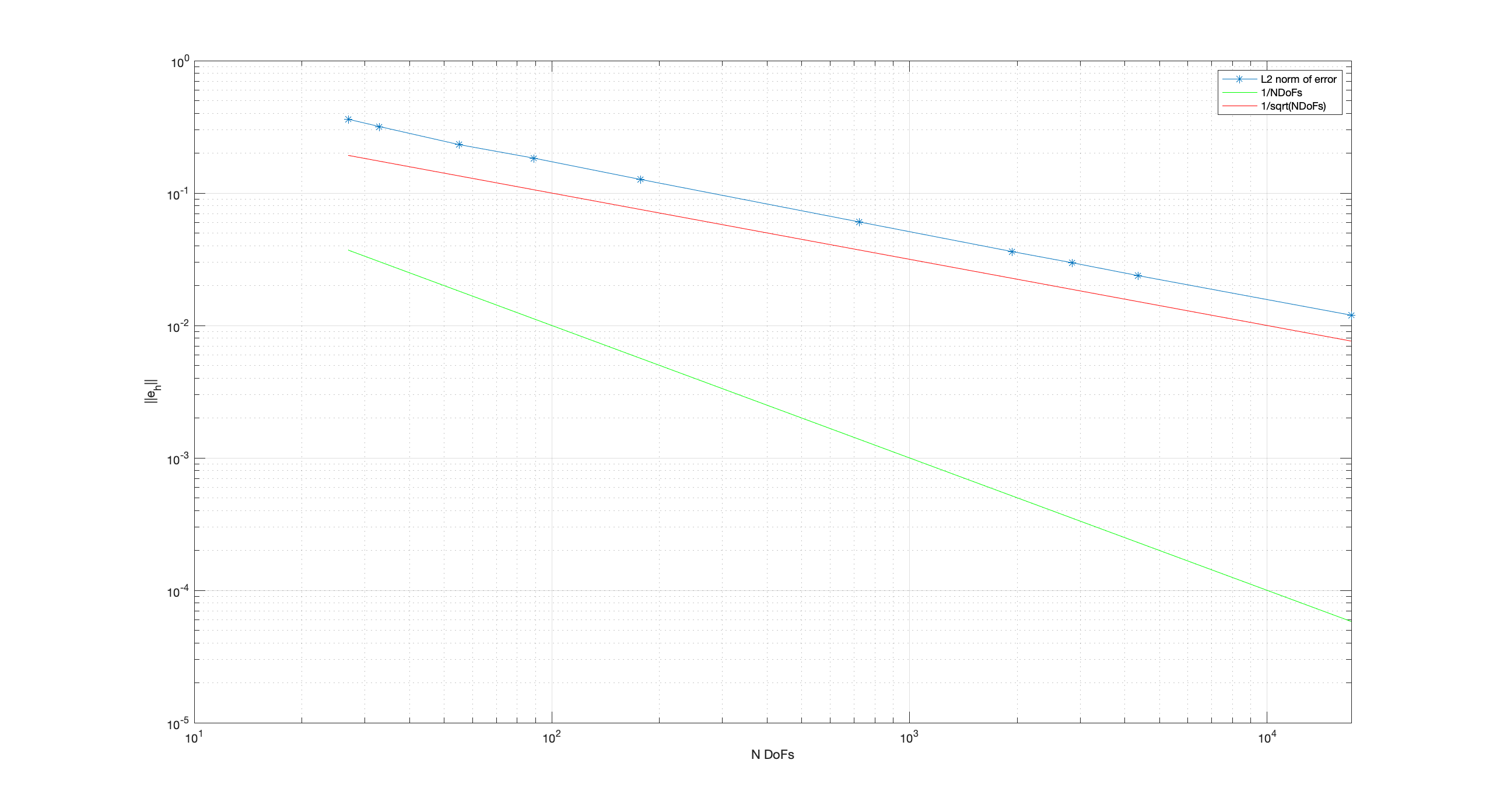
• Crucially, I noticed that in my reference paper for the implementation, the formula $(8)$ for $b_j^K$ is not what they implemented, since if you go to the first snippet, you may see that they multiplied by detJ the entries of $B$, while in that formula they divide their divergence by detJ. I don't know why, but if I do not multiply by detJ, I obtain the correct solution, as can be seen by the following graph for the pressure, and the correct $L^2$ convergence for the pressure (order $1$, as I am using 1 DoF per triangle).

[![enter image description here][2]][2]

function [A,B,F] = assemble(p,t,t2e,force)
[rspoints,qwgts] = GaussPoints(4);
nt = size(t,2); %N_triangles
ne = max(t2e(:)); %N_edges
A = sparse(ne,ne); %N_edges x N_edges
B = sparse(nt,ne); % N_triangles x N_edges
F = zeros(nt,1); %N_triangles

for K=1:nt
    l2g = t(1:3,K); %global node indices for element K
    edges = t2e(K,:);%global edges indices for element K
    tmp = l2g([2 3 1]) - l2g([3 1 2]);
    signs = tmp ./ abs(tmp);
    
    x = p(1,l2g); %x coords
    y = p(2,l2g); %y coords
    
    BK = [x(2)-x(1), x(3)-x(1);y(2)-y(1),y(3)-y(1)];
    bK = [x(1);y(1)];
    detBK = det(BK);
    
    detBK_inv = 1/abs(detBK);
    %% Loop over quadrature points
    for q=1:length(qwgts)
        r = rspoints(q,1); %x coordinate q-th quadrature point
        s = rspoints(q,2); %y coordinate q-th quadrature point
        [phi,divphi] = RT_shapes(r,s);
        
        JxW=qwgts(q)*detBK;
        physical_coords = BK*[r;s] + bK; %physical coordinates of the current quadrature points
        xp = physical_coords(1);
        yp = physical_coords(2);
        
        val_rhs = -force(xp,yp)*1.0*JxW;
        F(K) = F(K) + val_rhs;
        
        
        for i=1:3
            for j=1:3
                val_A =  detBK_inv*dot(signs(i)*BK*phi(:,i),signs(j)*BK*phi(:,j))*qwgts(q);
                A(edges(i),edges(j)) = A(edges(i),edges(j)) + val_A;
                
            end
            val_B = -signs(i)*divphi(i)*qwgts(q);
            B(K,edges(i)) = B(K, edges(i)) + val_B;
            
        end
        
        
    end
    
end