added 4318 characters in body
Source Link
Jamie
  • 121
  • 2

EDIT:

As per requested here's the full description of my MMS test with results:

I) As an initial step I solved the linear Poisson's equation with the rescaled Chebyshev derivatives: $$ \nabla^2 u = S $$ where BCs are periodic in x and zero Dirichlet in y as $u(x,a)=0$ & $u(x,b)=0$.

For the simple above case the test I performed with the MMS is: $$ u(x,y)=(y-a)(y-b)\sin{Ax} $$ while $n(x,y)$ was set to 1, the above case works perfectly for me and I have no issue at all. The results of this case are the following: enter image description here As you see above the numerical matches the exact solution for different domain lengths: $L_x=32; L_y=32,64,96,..$ and the adjusted code would be:
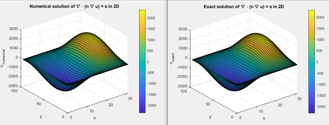
Nx = 4*16; 
Ny = 4*16; 
Lx =2*16;
kx  = fftshift(-Nx/2:Nx/2-1); % wave number vector
dx = Lx/Nx; 
% Use approximations for kx, and k^2. These come from Birdsall and Langdon
ksqu = (sin( kx * dx/2)/(dx/2)).^2 ;
kx = sin(kx * dx) / dx;
ksqu4inv = ksqu; 
ksqu4inv(abs(ksqu4inv)<1e-14) =1; %helps with error: matrix ill scaled because of 0s
xi_x =  2*pi/Lx;
xi  = (0:Nx-1)/Nx*2*pi;
x =  xi/xi_x;

ylow = 0;  %a
yupp =16;  %b
Ly = (yupp-ylow);
eta_ygl  = 2/Ly;
[D,etagl] = cheb(Ny);
% rescaling my Chebyshev Differentiation Matrices to an arbitrary domain [a,b] by performing a change of variables as the following:
ygl = (1/2)*((yupp-ylow)*etagl + (yupp+ylow));
D   = D*eta_ygl;
D2  = D*D;
[X,Y]   = meshgrid(x,ygl);

Igl = speye(Ny+1);
%ZNy represents the operation of setting the boundary values of y component
%to zero:
ZNy = diag([0 ones(1,Ny-1) 0]); %diag([0 ones(1,Ny-1) 0]); 
div_y_act_on_grad_y = D2* ZNy; 
%ICs
A = 2*pi / Lx;
u = (Y-ylow) .* (Y-yupp) .* sin( (A) * X);
uh = fft(u,[],2);

n = ones(size(u)); %set to 1
invnek = fft(1./n,[],2);
nh = fft(n,[],2);
dnhdxk = (kx*1i*xi_x).*nh;
dnhdyk =D * nh;

%Linear Exact source 
 LExactSource = (4*pi^2*(ylow-Y).*(Y-yupp).*sin(A*X))/Lx^2 + 2*sin(A*X);

oldSol = ones(size(u));
oldSolk = fft(oldSol ,[],2);
err_max =1e-4;
max_iter = 500;
Sourcek = fft(LExactSource ,[],2); 
for iterations = 1:max_iter
    oldSolMax = max(max(abs(oldSolk)));
    dudxk = (kx*1i*xi_x) .*oldSolk;
    %product:
    gradNgradUx = aapx(dnhdxk,dudxk);
    dudyk = (D) *oldSolk ; 
    gradNgradUy = aapx(dnhdyk,dudyk); 
    %RHS of PDE
    RHSk = Sourcek - (gradNgradUx + gradNgradUy); 
    Stilde = aapx(invnek,RHSk);
    for m = 1:length(kx)
        L = -Igl * (ksqu4inv(m))*xi_x^2+ div_y_act_on_grad_y;
        newSolk(:,m) = L\(Stilde(:,m));

    end
        %enforce BCs    
        newSolk=[zeros(1,Nx);  newSolk(2:Ny,:); zeros(1,Nx)];

    newSolMax = max(max(abs(newSolk)));
    if newSolMax < err_max 
        it_error = err_max /2;
    else
        it_error = abs( newSolMax - oldSolMax ) / newSolMax ;
    end
    if it_error < err_max
        break;
    end
    oldSolk = newSolk;

end
%plot numerical solution vs exact
 newSol= real(ifft(newSolk,[],2)); 
 figure
 surf(X, Y, newSol);
 colorbar;
 figure
 surf(X, Y, u);
 colorbar;

II) However, when I try to do the same for the nonlinear Poisson's equation with following expression: $$ \nabla \cdot (n\nabla u) = S $$ or can be expanded as: $n \nabla^2 u + \nabla u \cdot \nabla n = S$

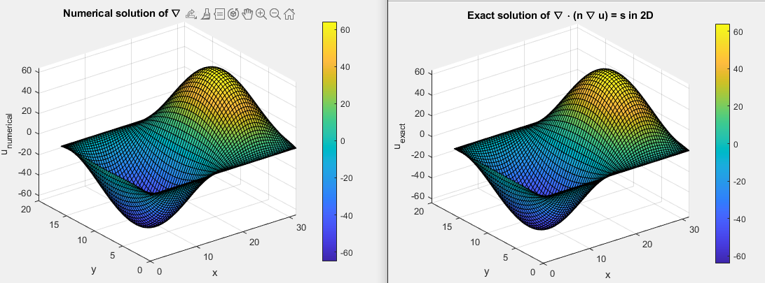
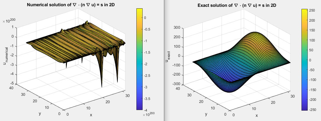
Then, using the MMS I chose $u(x,y)$ and $n(x,y)$ similarly as the first case: $$ u(x,y)=(y-a)(y-b)\sin{Ax} $$ $$ n(x,y)=\left(\frac{2}{b-a}\right)\left[y-\left(\frac{a+b}{2}\right) \right]^2\sin{3Ax}+10 $$ For the above nonlinear case with $L_x=32, L_y=16$ I get the following results: enter image description here However, if I change my domain length along y$L_x=32L_y=32$ this results in the solution blowing up as the following: enter image description here So, basically for the nonlinear case the code works for $L_y$ from 0 to 16 then blows up! I don't seem to see a pattern to begin to understand where the issue maybe. I have done an order of accuracy test where $L_x=L_y=16$ (case where solution does NOT blow up) and it gives me expected order of accuracy so any insight here would be helpful.

Source Link
Jamie
  • 121
  • 2

Where is the issue in my nonlinear PDE solver using pseudo-spectral methods with Chebyshev collocation?

This is a repost from another community, I think the question would be better here.

This bug has been haunting me for a while and would love new pair of eyes to help, not sure if this is the right place for such a question so please let me know.

I am solving a nonlinear Poisson's equation numerically using a mixed Chebyshev/Fourier spectral methods. Thus, assuming x is periodic and y is nonperiodic. I am trying to test my current numerical method/solver by using the method of manufacturing solution (MMS). Additionally, I am applying some coordinate mapping or rescaling my Chebyshev Differentiation Matrices to an arbitrary domain [a,b] by performing a change of variables as the following:

enter image description here

Thus, my chebyshev derivatives can be rewritten as:

enter image description here

The two above expressions were taken from the Weideman and Reddy paper found in this post:

Are there any alterations for the Chebyshev Differentiation Matrices on an arbitrary domain [a,b]?

My BCs are periodic in x and zero Dirichlet in y as $u(x,a)=0$ & $u(x,b)=0$.

Here is a simple example of my code with a simple MMS case of a non-linear Poisson's equation:

Nx = 4*16; 
Ny = 4*16; 
Lx =2*16;
kx  = fftshift(-Nx/2:Nx/2-1); % wave number vector
dx = Lx/Nx; 
% Use approximations for kx, and k^2. These come from Birdsall and Langdon
ksqu = (sin( kx * dx/2)/(dx/2)).^2 ;
kx = sin(kx * dx) / dx;
ksqu4inv = ksqu; 
ksqu4inv(abs(ksqu4inv)<1e-14) =1; %helps with error: matrix ill scaled because of 0s
xi_x =  2*pi/Lx;
xi  = (0:Nx-1)/Nx*2*pi;
x =  xi/xi_x;

ylow = 0;  %a
yupp =16;  %b
Ly = (yupp-ylow);
eta_ygl  = 2/Ly;
[D,etagl] = cheb(Ny);
% rescaling my Chebyshev Differentiation Matrices to an arbitrary domain [a,b] by performing a change of variables as the following:
ygl = (1/2)*((yupp-ylow)*etagl + (yupp+ylow));
D   = D*eta_ygl;
D2  = D*D;
[X,Y]   = meshgrid(x,ygl);

Igl = speye(Ny+1);
%ZNy represents the operation of setting the boundary values of y component
%to zero:
ZNy = diag([0 ones(1,Ny-1) 0]); %diag([0 ones(1,Ny-1) 0]); 
div_y_act_on_grad_y = D2* ZNy; 
%ICs
A = 2*pi / Lx;
u = (Y-ylow) .* (Y-yupp) .* sin( (A) * X);
uh = fft(u,[],2);

n = (eta_ygl)*(Y-((ylow+yupp)/2)).^2 .* sin( (3 * A) * X)+ 10;
invnek = fft(1./n,[],2);
nh = fft(n,[],2);
dnhdxk = (kx*1i*xi_x).*nh;
dnhdyk =D * nh;

%Exact source 
 ExactSource = (1/(2*(ylow - yupp)))*((-2 + ylow*A^2 *(yupp - Y) + A^2 .*Y .*(-yupp + Y)) .*sin(A*X) .*(20*(-ylow + yupp) + (ylow + yupp - 2*Y).^2 .* sin(3*A*X)) - (ylow + yupp - 2*Y).^2 .*(3*A^2 *(ylow - Y) .* (yupp - Y) .* cos(A *X).^2 .* (-1 + 2*cos(2*A*X)) + 4*sin(A*X) .*sin(3*A*X)));

oldSol = ones(size(u));
oldSolk = fft(oldSol ,[],2);
err_max =1e-4;
max_iter = 500;
Sourcek = fft(ExactSource,[],2); 
for iterations = 1:max_iter
    oldSolMax = max(max(abs(oldSolk)));
    dudxk = (kx*1i*xi_x) .*oldSolk;
    %product:
    gradNgradUx = aapx(dnhdxk,dudxk);
    dudyk = (D) *oldSolk ; 
    gradNgradUy = aapx(dnhdyk,dudyk); 
    %RHS of PDE
    RHSk = Sourcek - (gradNgradUx + gradNgradUy); 
    Stilde = aapx(invnek,RHSk);
    for m = 1:length(kx)
        L = -Igl * (ksqu4inv(m))*xi_x^2+ div_y_act_on_grad_y;
        newSolk(:,m) = L\(Stilde(:,m));

    end
        %enforce BCs    
        newSolk=[zeros(1,Nx);  newSolk(2:Ny,:); zeros(1,Nx)];
    
    newSolMax = max(max(abs(newSolk)));
    if newSolMax < err_max 
        it_error = err_max /2;
    else
        it_error = abs( newSolMax - oldSolMax ) / newSolMax ;
    end
    if it_error < err_max
        break;
    end
    oldSolk = newSolk;
 
end
%plot numerical solution vs exact
 newSol= real(ifft(newSolk,[],2)); 
 figure
 surf(X, Y, newSol);
 colorbar;
 figure
 surf(X, Y, u);
 colorbar;

Cheb(N) function is taken from Spectral Methods textbook and can be found: HERE

% CHEB compute D = differentitation matrix, x = Chebyshev grid
function [D, x] = cheb(N)
  if N == 0, D = 0; x = 1; return, end
  x = cos(pi*(0:N)/N)';
  c = [2; ones(N-1,1); 2].*(-1).^(0:N)';
  X = repmat(x,1,N+1);
  dX = X-X';
  D = (c*(1./c)')./(dX+(eye(N+1)));
  D = D - diag(sum(D'));

and aapx is a function deals with aliasing errors:

function ph=aapx(uh,vh) %anti-aliased product, 
% in: uh,vh from fft with n samples
%use discrete transform with m rather than n points, where m >= 3N/2
[ny nx]=size(uh);m=nx*3/2;
uhp=[uh(:,1:nx/2) zeros(ny,(m-nx)) uh(:,nx/2+1:nx)]; % pad uhat with zeros
vhp=[vh(:,1:nx/2) zeros(ny,(m-nx)) vh(:,nx/2+1:nx)]; % pad vhat with zeros
up=ifft(uhp,[],2); 
vp=ifft(vhp,[],2); 
w=up.*vp; 
wh=fft(w,[],2);
ph=1.5*[wh(:,1:nx/2) wh(:,m-nx/2+1:m)]; % extract F-coefficients 

The issue is this code works for "certain" domain lengths and blows up for others. For example, it works fine for Lx=Ly=16 and breaks for Lx=16, and Ly=32. I have ran many debugging tests to no avail. I don't see the issue at all and the code returns no error messages to work with. Would love some feedback on how to tackle this. Thanks!