The most important aspect of interpolation and curve fitting is to understand why high order polynomial fits can be an issue and what the other options are and then you can understand when they are/are not a good choice.
A few issues with high order polynomials:
Polynomials are naturally oscillatory functions. As the order of the polynomial increases, the number of oscillations increases and these oscillations become more severe. I'm simplifying here, the possibility of multiple and imaginary roots makes it a bit more complex, but the point is the same.
Polynomials approach +/- infinity at a rate equal to the polynomial order as x goes to +/- infinity. This is often not a desired behavior.
Computing polynomial coefficients for high order polynomials is typically an ill conditioned problem. This means that small errors (such as rounding in your computer) can create large changes in the answer. The linear system that must be solved involves a Vandermonde Matrix which can easily be ill conditioned.
I think that perhaps the heart of this issue is the distinction between curve fitting and interpolation.
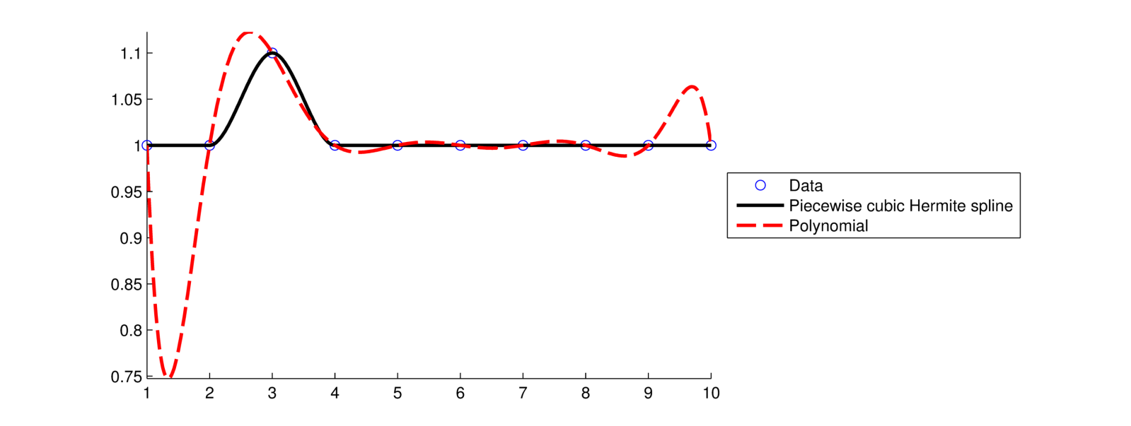
Interpolation is used when you believe that your data is very accurate so you want your function to exactly match the data points. When you need values between your data points it's typically best to use a smooth function that matches the local trend of the data. Cubic or Hermite splines are often a good choice for this type of problem since they are much less sensitive to non-local (meaning at data points far away from a given point) changes or errors in the data and are less oscillatory than a polynomial. Consider the following data set:
x = 1   2   3   4   5   6   7   8   9  10
y = 1   1 1.1   1   1   1   1   1   1   1

A polynomial fit has much larger oscillations, especially near the edges of the data set, than a Hermite spline.
On the other hand, least squares approximation is a curve fitting technique. Curve fitting is used when you have some idea of the expected functionality of your data, but you don't need your function to exactly pass through all the data points. This is typical when the data may contain measurement errors or other imprecisions or when you wish to extract the general trend of the data. Least squares approximation is most often introduced in a course by using polynomials for the curve fitting because this results in a linear system that is relatively simple to solve using the techniques you likely learned earlier in your course. However, least squares techniques are much more general than just polynomial fits and can be used to fit any desired function to a data set. For example, if you expect an exponential growth trend in your data set, you can fit an exponential curve using least squares or linearized least squares.
Finally, choosing the correct function to fit your data is as important as correctly performing the interpolation or least squares computations. Doing so even allows the possibility of (cautious) extrapolation. Consider the following situation. Given population data (in millions of people) for the US from 2000-2010:
Year:  2000   2001   2002   2003   2004   2005   2006   2007   2008   2010
Pop.: 284.97 287.63 290.11 292.81 295.52 298.38 301.23 304.09 306.77 309.35
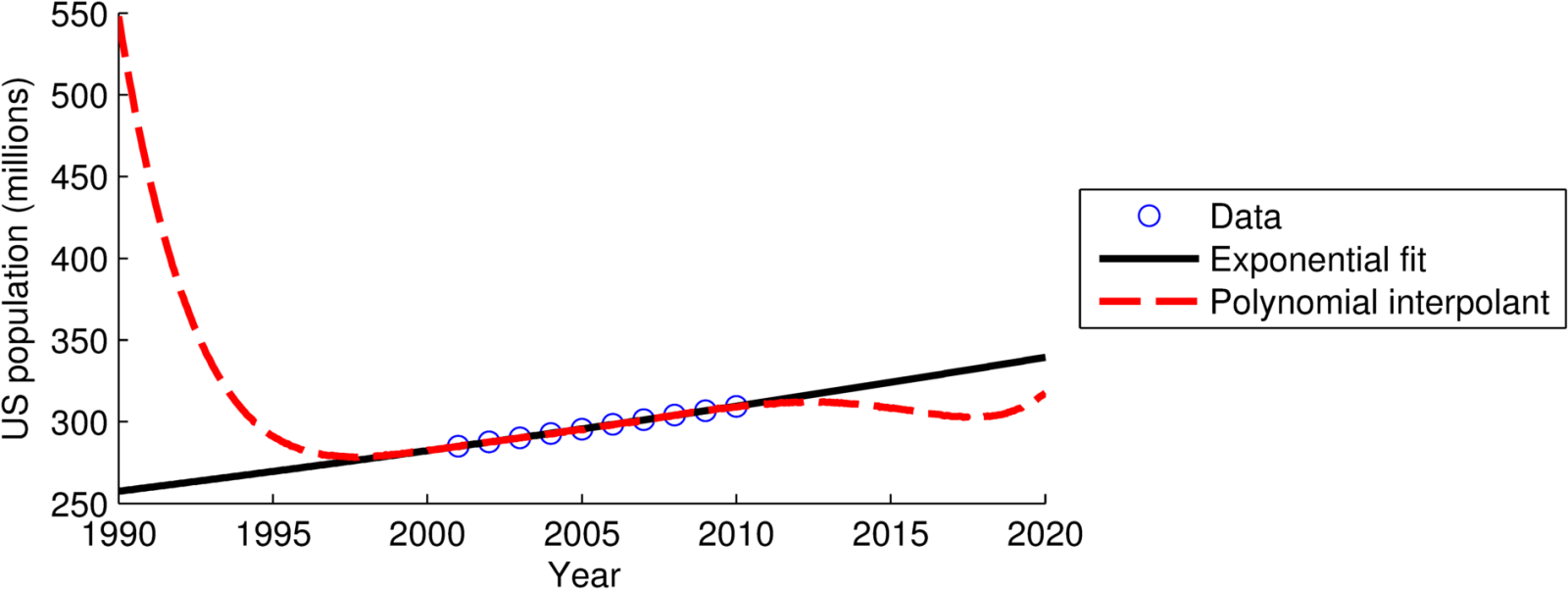
Using an exponential linearized least squares fit N(t)=A*exp(B*t) or a 10th order polynomial interpolant gives the following results:

US population growth is not quite exponential, but I'll let you be the judge of the better fit.

