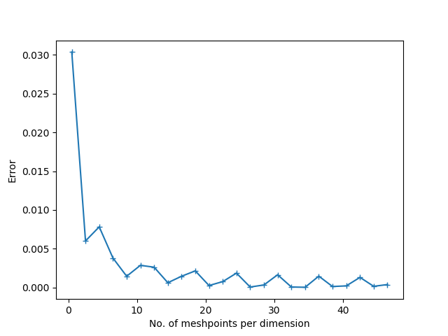
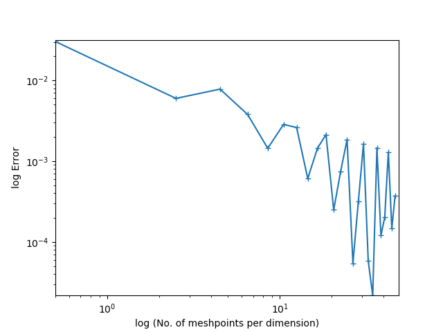
While I cannot comment your particular case as you didn't provide enough details, I can give some guidance on the matter since I've spent several years of my life trying to make these convergence graphs look as nice as possible. I've only worked with elliptic and saddle-point problems and the guidance probably doesn't apply to parabolic and hyperbolic problems at all.
One thing should be clear already from the comments: there is no reason whatsoever for the graphs to always look like straight lines if you have an upper bound for the error.
Another thing to realize is that such error estimates are usually satisfied by some generic set of problems where the boundary and loading data is specified as an element of a Sobolev space. Thus, there are in reality lots of problems with different loadings, boundary conditions, etc. that satisfy the same estimate—typically with a different constant. When numerically solved on a sequence of meshes, only some of the problems stay near enough the asymptotic limit—as defined by the estimate—for the graphs to look linear.
A third thing to notice is that many times you have multiple asymptotic limits in place, e.g., from different boundary conditions, singularities, and varying regularity of the data. Obviously the estimate with the smallest power of $h$ will dominate in the limit $h \rightarrow 0$ but it is sometimes hard to know that when the other estimates still have an effect. This range where the non-dominating estimates still have an effect is sometimes referred to as the preasymptotic range.
Artificially making the preasymptotic range as small as possible and finding problems that mainly stay near the asymptotic limit is more of an art than a science. Here are some tips:
- Make sure that the initial mesh is refined enough to reasonably represent all the nonlinearities in the data. For example, if the loading or boundary condition has $\sin(x)$, make sure that $h << \pi$.
- Make sure that there are no singularities other than the ones that you're interested in studying.
- Make sure that you don't make any accidental variational crimes, e.g., integrate all functions and data exactly if possible. If not possible, use at least $L^2$ projection to define the boundary and loading data. Be careful with low regularity data, i.e. discontinuous data. Be extra careful also when integrating non-polynomial data.
- Make sure that the sequence of meshes is nested. This will often improve the monotonicity of the graph: the next mesh should always be better than the previous one.
- Make sure you use high enough integration rule when evaluating the error. I've made this mistake more than once and it took a while to realize where the problem was.
- Don't use integration points that reside on element boundaries if you have discontinous data over the element boundary. I've also made this mistake once and it took a while to debug.
In general, I think the error estimates are more useful when checking that your newly implemented finite element code is working correctly and not so useful for applied problems where the data and the boundary conditions are not necessarily nice enough for you to get linear convergence graphs.
If you provide more details on the problem at hand, I think I could provide more specific tips. However, I think these tips will get you started on finding the problem.

