How to generate the convolution of f(x, y) with a parametric function g(t), x(t), y(t) in Python? (Something better than this brute-force sum)

Question

The answer to Convolute a gaussian kernel with a large array of off-grid centroids without looping? (how to make "A Thousand (Gaussian) Points of Light" ) involves summing a 3D array over its stacked direction. This question however is about convolution using continuous functions rather than summation.

The answer there mentions

a Fredholm integral equation of the first kind

and that may work here as well.

---

I'd like to know how to convolute $f(x, y)$ with a parametric shape; a 1D distribution along a parametric path as defined by $g(t), \ x(t), \ y(t)$ in Python, resulting in a 2D array of $f * g$.

A simple, illustrative example of this would be:

$$g(t) = \frac{\Gamma^2}{(t-t_0)^2 + \Gamma^2} \ \ \ \text{ (the 1D function)}$$

$$x(t), \ y(t) = a\cos(t), \ a\sin(t) \ \ \ \text{ (over the 2D path)}$$

$$f(x, y) = \exp(-(x^2+y^2)/2 \sigma^2) \ \ \ \text{ (the 2D kernel)}$$

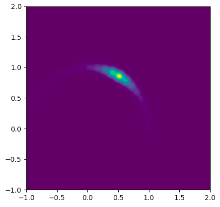
If $a=1, \ t_0 = \pi/3, \ \Gamma = \pi/30 \text{ and } \sigma=0.05$ then I can approximate it brute force as follows; I've made the parametric variable $t$ step size large intentionally to illustrate the sum. Making it sufficiently densely spaced to reduce the error in the result and adding the appropriate normalization (omitted here) is the brute-force solution, I'm wondering if I'm missing a simpler solution that might be better in cases where the parametric function is longer and more complicated.

note: "Better" in this case means faster, as in running mostly in compiled code of some Python method or library; this calculation will be done perhaps 100 times each time a user touches a slider in an interactive simulation.

import numpy as np
import matplotlib.pyplot as plt

t_0 = np.pi/3
gamma = np.pi/20
a = 1.
sigma = 0.05

all_t = np.linspace(0, 2*np.pi, 50) # big steps to make it bumpy
all_g = gamma**2 / ((all_t - t_0)**2 + gamma**2)

y, x = np.mgrid[-1:2:501j, -1:2:501j]

result = np.zeros_like(y)
for (yc, xc), g in zip(zip(*[a * f(all_t) for f in (np.sin, np.cos)]), all_g):
    result += g * np.exp(-((x-xc)**2 + (y-yc)**2)/(2*sigma**2))

extent = [x.min(), x.max(), y.min(), y.max()]
plt.imshow(result, origin='lower', extent=extent)
plt.show()
    

Answer 1

Not stating that this approach is faster, but maybe it inspires you or someone else. The conventional approach in here was certainly faster compared to my implementation of the approach outlined below. My goal was to somehow combine the parameterized path $(\varphi_1(t),\varphi_2(t))$ and $g(t)$ into a single entity.

Taking the parameterized path as $\varphi_1(t)$ and $\varphi_2(t)$, the expression for the convolution is: \begin{align} q(x,y) &= \int_{0}^{2\pi} e^{-b((x-\varphi_1(t))^2 + (y-\varphi_2(t))^2)}g(t) \text{d}t\\ &= e^{-b(x^2+y^2)}\int_{0}^{2\pi}e^{2bx\varphi_1(t)}e^{2by\varphi_2(t)}g(t)e^{-b(\varphi_1^2(t)+\varphi_2^2(t))} \text{d}t \end{align} Then defining $$\hat{g}(t) = g(t)e^{-b(\varphi_1^2(t)+\varphi_2^2(t))}$$ and using Taylor expansions of the exponential functions \begin{align} q(x,y) &= e^{-b(x^2+y^2)}\sum_{h=0}^{\infty}\sum_{k=0}^{\infty} \frac{(2bx)^k}{k!}\frac{(2by)^h}{h!}\int_{0}^{2\pi}\varphi_1^k(t)\varphi_2^h(t)\hat{g}(t)\text{d}t \end{align} The integral can be rearranged into a matrix $G$ with components $G_{kh}$ \begin{align} G_{kh}=\int_{0}^{2\pi}\varphi_1^k(t)\varphi_2^h(t)\hat{g}(t)\text{d}t \end{align} Thus, the path $(\varphi_1(t),\varphi_2(t))$ and $g(t)$ are encoded in $G$.

The double sum can be rewritten as: \begin{align} \hat{x}^TG\hat{y} = \sum_{h=0}^{H}\sum_{k=0}^{K} \frac{(2bx)^k}{k!}\frac{(2by)^h}{h!}\int_{0}^{2\pi}\varphi_1^k(t)\varphi_2^h(t)\hat{g}(t)\text{d}t \end{align} With $\hat{x}$ and $\hat{y}$ being a vectors with components corresponding to different $k$ and $h$, i.e. $$\hat{x}_k = \frac{(2bx)^k}{k!}\,\,\,\,\,\,\,\,\,\,k=0,1,2,3,4...$$ $$\hat{y}_h = \frac{(2by)^h}{h!}\,\,\,\,\,\,\,\,\,\,h=0,1,2,3,4...$$ For proper computation of the components, Stirling's formula may be used.

Then the convolution $q(x,y)$ can be written as $$q(x,y)=\hat{x}^TG\hat{y} e^{-b(x^2+y^2)}$$ I tried it out in Matlab and it works, though it's rather slow. Maybe it can be done faster.