For noisy or fine-structured data, are there better quadratures than the midpoint rule?

Question

Only the first two sections of this long question are essential. The others are just for illustration.

Background

Advanced quadratures such as higher-degree composite Newton–Cotes, Gauß–Legendre, and Romberg seem to be mainly intended for cases where one can finely sample the function but not integrate analytically. However, for functions with structures finer than the sampling interval (see Appendix A for an example) or measurement noise, they cannot compete with simple approaches such as the midpoint or trapezoid rule (see Appendix B for a demonstration).

This is somewhat intuitive as, e.g., the composite Simpson rule essentially “discards” one quarter of the information by assigning it a lower weight. The only reason such quadratures are better for sufficiently boring functions is that properly handling border effects outweighs the effect of discarded information. From another point of view, it is intuitively clear to me that for functions with a fine structure or noise, samples that are remote from the borders of the integration domain must be almost equidistant and have almost the same weight (for a high number of samples). On the other hand, quadrature of such functions may benefit from a better handling of border effects (than for the midpoint method).

Question

Assume that I wish to numerically integrate noisy or fine-structured one-dimensional data.

The number of sampling points is fixed (due to function evaluation being costly), but I can freely place them. However, I (or the method) cannot place sampling points interactively, i.e., based on results from other sampling points. I also do not know potential problem regions beforehand. So, something like Gauß–Legendre (non-equidistant sampling points) is okay; adaptive quadrature is not since it requires interactively placed sampling points.

• Have any methods going beyond the midpoint method been suggested for such a case?

• Or: Is there any proof that the midpoint method is best under such conditions?

• More generally: Is there any existing work on this problem?

Appendix A: Specific example of a fine-structured function

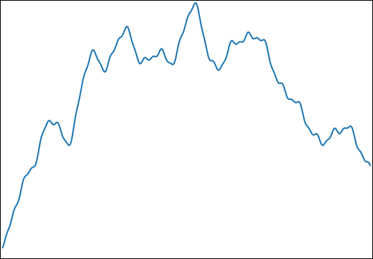
I wish to estimate $\int_0^1f(t)\, \mathrm{d}t$ for: $$ f(t) = \sum_{i=1}^{k} \frac{\sin(ω_i t-φ_i)}{ω_i},$$ with $φ_i∈ [0,2π]$ and $\log{ω_i} ∈ [1,1000]$. A typical function looks like this:

I chose this function for the following properties:

• It can be integrated analytically for a control result.
• It has fine structure on a level that makes it impossible to capture all of it with the number of samples I am using ($<10^2$).
• It is not dominated by its fine structure.

Appendix B: Benchmark

For completeness, here is a benchmark in Python:

import numpy as np
from numpy.random import uniform
from scipy.integrate import simps, trapz, romb, fixed_quad

begin = 0
end   = 1

def generate_f(k,low_freq,high_freq):
    ω = 2**uniform(np.log2(low_freq),np.log2(high_freq),k)
    φ = uniform(0,2*np.pi,k)
    g = lambda t,ω,φ: np.sin(ω*t-φ)/ω
    G = lambda t,ω,φ: np.cos(ω*t-φ)/ω**2
    f = lambda t: sum( g(t,ω[i],φ[i]) for i in range(k) )
    control = sum( G(begin,ω[i],φ[i])-G(end,ω[i],φ[i]) for i in range(k) )
    return control,f

def midpoint(f,n):
    midpoints = np.linspace(begin,end,2*n+1)[1::2]
    assert len(midpoints)==n
    return np.mean(f(midpoints))*(n-1)

def evaluate(n,control,f):
    """
    returns the relative errors when integrating f with n evaluations
    for several numerical integration methods.
    """
    times = np.linspace(begin,end,n)
    values = f(times)
    results = [
            midpoint(f,n),
            trapz(values),
            simps(values),
            romb (values),
            fixed_quad(f,begin,end,n=n)[0]*(n-1),
        ]

    return [
            abs((result/(n-1)-control)/control)
            for result in results
        ]

method_names = ["midpoint","trapezoid","Simpson","Romberg","Gauß–Legendre"]

def med(data):
    medians = np.median(np.vstack(data),axis=0)
    for median,name in zip(medians,method_names):
        print(f"{median:.3e}   {name}")

print("superimposed sines")
med(evaluate(33,*generate_f(10,1,1000)) for _ in range(100000))

print("superimposed low-frequency sines (control)")
med(evaluate(33,*generate_f(10,0.5,1.5)) for _ in range(100000))

(I here use the median to reduce the influence of outliers due to functions that have only high-frequency content. For the mean, the results are similar.)

The medians of the relative integration errors are:

superimposed sines
6.301e-04   midpoint
8.984e-04   trapezoid
1.158e-03   Simpson
1.537e-03   Romberg
1.862e-03   Gauß–Legendre

superimposed low-frequency sines (control)
2.790e-05   midpoint
5.933e-05   trapezoid
5.107e-09   Simpson
3.573e-16   Romberg
3.659e-16   Gauß–Legendre

Note: After two months and one bounty without result, I posted this on MathOverflow.

Answer 1

First of all, I think you misunderstand the concept of adaptive quadrature. Adaptive quadrature does not imply "interactively placing sample points". The whole idea behind adaptive quadrature is to devise a scheme that will integrate a certain function to a certain (estimated) absolute or relative error with as little function evaluations as possible.

A second remark: you write "The number of sampling points is fixed (due to function evaluation being costly), but I can freely place them". I think the idea should be that the number of sampling points (or function evaluations in quadrature terminology) should be as small as possible (i.e. not fixed).

So what is the idea behind adaptive quadrature as implemented in QUADPACK for example?

1. The basic ingredient is a "nested" quadrature rule: this is a combination of two quadrature rules where one has a higher order (or accuracy) as the other. Why? Based on the difference between these rules, the algorithm can estimate the quadrature error (of course, the algorithm will use the most accurate one as the reference result). Examples could be the trapezoid rule with $2^{n}$ nodes and $2^{n+1}$ nodes. In the case of QUADPACK, the rules are Gauss-Kronrod rules. These are interpolatory quadrature rules that use a Gauss-Legendre quadrature rule of a certain order $N$ and an optimal extension of this rule. This means that a higher quadrature order can be obtained by re-using the Gauss-Legendre nodes (i.e. the costly function evaluations) with different weights and adding a number of extra nodes. In other words, the original Gauss-Legendre rule of order $N$ will integrate all polynomials of degree $2N-1$ exactly while the extended Gauss-Kronrod rule will integrate some higher order polynomial exactly. A classic rule is the G7K15 (7th order Gauss-Legendre with 15th order Gauss-Kronrod). The magic is that the 7 nodes of the Gauss-Legendre are a subset of the 15 nodes of the Gauss-Kronrod so with 15 function evaluations, I have a quadrature evaluation together with an error estimate!

2. Next ingredient is a "divide-and-conquer" strategy. Suppose you let loose this G7K15 on your integrand and you observe a quadrature error that is according to your taste too large. QUADPACK will then subdivide the original interval in two equally spaced subintervals. And then it will re-evaluate the two subintegrals using the basic rule, G7K15. Now, the algorithm has a global error estimate (which should be hopefully lower than the first one) but also two local error estimates. It picks the interval with the largest error and divides this one in two. Two new integrals are estimated and the global error is updated. And so on until the global error is below your requested target or the maximum number of subdivisions has been surpassed.

So I challenge you to update your code above using the scipy.quad method. Maybe in case of an integrand with a lot of "fine structure" you might need to increase the maximum number of subdivisions (the limit option). You could also play with the epsabs and/or epsrel parameters.

However, if you only have experimental data, I see two possibilities.

1. If you have the opportunity to select the measurement points, i.e. values of $t$, I would select them equidistanly and preferably as a power of $2$ so that you can apply a nested trapezoidal rule (and profit from Romberg extrapolation).
2. If you have no means of choosing the nodes, i.e. the measurements come at random times, the best option in my opinion still is the trapezoid rule.

Answer 2

I am not convinced that your code demonstrates anything fundamental about the various quadrature rules and how well they do against noise and fine structure, and believe it likely that if you chose various different fines structure you would find something different. Here's the theorem:

No quadrature method can give low absolute or relative error against a function with unbounded total variation. In a floating point system with unit roundoff $\mu$, we have the estimate $$ \left| \int_{a}^{b} f \, \mathrm{d}x - \hat{Q}[\hat{f}] \right| \le \left| \int_{a}^{b} f \, \mathrm{d}x - Q[f] \right| + \mu\left[ 4\int_{a}^{b} |f| \, \mathrm{d}x + \int_{a}^{b} |xf'| \, \mathrm{d}x \right] $$ where $\hat{Q}$ is the quadrature sum acting on the numerical implementation $\hat{f}$ of $f$.

Proof: Let the quadrature nodes be $\{x_i\}_{i=0}^{n-1}$ and the (non-negative) quadrature weights be $\{w_i\}_{i=0}^{n-1}$ and denote their floating point approximations by $\hat{w}_{i}$ and $\hat{x}_i$. Assume that $\hat{f}$ satisfies $\hat{f}(x) = f(x)(1+2\delta)$ where $|\delta| \le \mu$ where $\mu$ is the unit roundoff. Then \begin{align*} \hat{Q}[\hat{f}] &= \sum_{i=0}^{n-1} \hat{w}_i \otimes \hat{f}(\hat{x}_i) \\ &= \sum_{i=0}^{n-1} w_i (1+\delta^w_i)f(x_i + \delta_i^x x_i)(1+2\delta_i^{f})(1+\delta_i^{*}) \\ &\approx \sum_{i=0}^{n-1} w_i \left[f(x_i)+ \delta_i^x x_i f'(x_i) \right] (1+\delta^w_i + 2\delta_i^{f} + \delta_i^*) \\ &\approx \sum_{i=0}^{n-1} w_i f(x_i) + \sum_{i=0}^{n-1}\delta_i^x w_i x_i f'(x_i) + w_i f(x_i) (\delta^w_i + 2\delta_i^{f} + \delta_i^*) \\ \end{align*} so that \begin{align*} |\hat{Q}[\hat{f}] - Q[f]| &\le \mu \sum_{i=0}^{n-1}w_i(|x_i f'(x_i)| + 4|f(x_i)|) \\ &\approx 4\mu \int |f| \, \mathrm{d}x + \mu \int |xf'| \, \mathrm{d}x \end{align*} This assumes that the sum is computed without error; multiply by $n$ to drop that assumption.

Mutatis mutandis you can also show that the result holds in fixed point arithmetic.