Singular values of $X$ in $AX+XA=C$?

Question

Suppose I have semi-positive definite matrices $A$ and $C$, is there an efficient approach to get top singular values of X entering the following expression?

$$ AX+XA=C $$

My matrices are 4k-by-4k and are known to be low rank, rank somewhere between 50 and 1000.

I've been using SVD on top of scipy.linalg.svd(scipy.linalg.solve_lyapunov(A, C)), but it's too slow for my application.

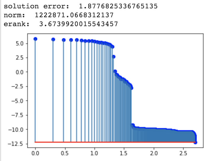
The second issue is the issue of stability. Using scipy.linalg to solve $AX+XA=2A$ gives me solution with norm much higher than 1 which I expected since $I=X$ is a valid solution. Since I'm interested in the spectrum, I may need some extra constraints to make this problem well defined. Also, there seems to be significant error introduced (plugging X into the equation and looking at norm gives me relative errors around 2)

https://colab.research.google.com/drive/113XQ88puFNNSQHPnO-zoAgm-8w01ANuh#scrollTo=n6OQHQ5jYw53

Background

These singular values come up in the problem of determining length of step size for linear least-squares estimation, described here: https://arxiv.org/abs/1610.03774

Suppose we are solving linear least squares problem in $d$ dimensions by minimizing the following objective:

$$L(w) = \frac{1}{2}E_{xy}[y-\langle w, x\rangle^2]$$ Residual is defined as $$\epsilon_{x,y}=y-\langle w, x\rangle$$

Hessian of this loss is $$H=E[xx']$$

While covariance matrix of gradients $$\Sigma = E[\epsilon_{xy} xx']$$

The problem is to minimize this loss using stochastic gradient descent. How big can we make the step size? We can show that when errors are uncorrelated with observations, following step size can be taken while still maintaining convergence

$$\gamma = \frac{2}{R^2}$$

where $R^2$ is an upper bound on $\|x\|^2$

However, when errors are correlated (heteroscedactic/misspecified case), this rate must be reduced to the following

$$\gamma = \frac{2}{\rho R^2}$$

Where $1\le \rho\le d$ is a measure of misspecification, and is computed as follows

Let $X$ be the solution of the following $$HX+XH=\Sigma$$

Then $$\rho=d \frac{\|X\|_2}{\text{tr}(X)}$$

The peculiarity of data generating process (these are features generated by neural network) means that $x$ lie in an unknown low-dimensional subspace of $\mathbb{R}^d$ . $d\in[4000,10000]$, but true dimensionality is 50-1000

The task is:

1. Compute $\rho$ efficiently in order to obtain step size to use for SGD
2. Compute full spectrum of $X$ efficiently for visualization purposes

Answer 1

The speed problem can be fixed: there is literature on methods for large and sparse Lyapunov equations that return $X \approx ZZ^T$ already in factored form (hence sparing you most of the work also in the SVD part). See for instance https://www.mpi-magdeburg.mpg.de/projects/mess and http://www.dm.unibo.it/~simoncin/software.html for the two leading methods.

But, first of all, you need to understand the issue with multiple solutions.

Answer 2

To address the singularity issue: have you thought about projecting the equation on $\operatorname{range}(A)$? Write $A= Q\hat{A}Q^T$, with $Q\in \mathbb{R}^{d\times k}$ a tall thin matrix with orthogonal columns ($Q^TQ=I$) and $\hat{A}\in\mathbb{R}^{k\times k}$ nonsingular, and accordingly $X=Q\hat{X}Q^T$. Then you can multiply the equation on the left and right by $Q^T$ and $Q$, to get the small-scale equation $$\hat{A}\hat{X}+\hat{X}\hat{A}=\hat{C},$$ with $\hat{C} = Q^TCQ$. This will give you a solution with $\operatorname{range}(X) \subseteq \operatorname{range}(A)$. Not sure if that makes sense in your application.

I did not check, but I would not be surprised if it turned out that this is the same solution as your rank-deficient least-squares approach.

Also, I guess you already have all the pieces available to compute the coefficients of the small-scale equation without even forming a single $d\times d$ matrix, just with a QR of the data matrix containing the vectors $x$.