Backwards Difference Implicit Method for Nonlinear Parabolic PDE in Python

Question

Original Stack Overflow Question: https://stackoverflow.com/questions/65683788/indexerror-index-31-is-out-of-bounds-for-axis-1-with-size-31?noredirect=1#comment116218335_65683788

PDE: u_t = u_xx + u(u_x)^2

The backward difference was used the time derivative meanwhile a central difference was used for the first space derivative.

If you follow the link you can see that I cannot get solutions that make sense and I cannot figure out how to. I'm adamant it is to do with the function f at the finite-difference algorithm stage. Currently, I understand that f is a vector and hence only generating the initial condition. But when I try something like f[1:M, q] it doesn't work.

Code:

import numpy as np
import matplotlib.pyplot as plt
from mpl_toolkits.mplot3d import Axes3D
from matplotlib import cm
import math
from scipy.sparse import spdiags
from numpy.linalg import inv

M = 30
dx = 1 / M
r = 0.25

tmax = 0.2
dt = r * dx**2
N = math.floor(tmax / dt)

x = np.linspace(0, 1, M + 1)
t = np.linspace(0, tmax, N + 1)


U = np.zeros((M + 1, N + 1))                           # Initial array for solution u(x, t)

U[:, 0] = 40 * x**2 * (1 - x) / 3                      # Initial condition 
U[0, :] = 0                                            # Boundary condition at x = 0
U[-1, :] = 0                                           # Boundary condition at x = 1 


for q in range(1, N):
    U[:, q+1] = U[:, q]
    for p in range(1, 10):
        f = np.zeros((M+1, M+1))
        for k in range(2, M):
            f = U[k, q+1] - r * (U[k+1, q+1] + U[k-1, q+1]) + 2 * r * U[k, q+1] \
              - r * U[k, q+1] * U[k+1, q+1]**2 + r * U[k+1, q+1]**2 * U[k, q+1] - r * U[k, q+1]**3


        updiag = -r - 2 * r * U[p, q + 1] * U[p+1, q + 1] + 2 * r * U[p, q + 1]**2
        diag = 1 + 2 * r + 3 * r * U[p, q + 1]**2 - 4 * r * U[p+1, q + 1] * U[p+1, q+1] - 2 * r * U[p, q + 1]**2
        lowdiag = r
        Jdata = np.array([31 * [diag], 31 * [lowdiag], 31 * [updiag]])
        Diags = [0, -1, 1]
        J = spdiags(Jdata, Diags, 31, 31).toarray()
        d = inv(J) * f
        u = U[:, q+1]
        u = u + d
        U[1, q + 1] = 0
        U[M, q + 1] = 0


T, X = np.meshgrid(t, x)

fig = plt.figure()
ax = fig.gca(projection='3d')

surf = ax.plot_surface(T, X, U, cmap=cm.coolwarm)

ax.set_xlabel('t')
ax.set_ylabel('x')
ax.set_zlabel('u(x, t)')

plt.tight_layout()
plt.savefig('BDImplSol.pdf', bbox_inches='tight')
plt.show()

Edit Discretisation formula:

$$ U_i^{n + 1} = U_i^n + r \left(\left(U_{i+1}^{n+1} - 2 U_i^{n+1} + U_{i-1}^{n+1} \right) + U_i^{n + 1} \left(U_{i + 1}^{n + 1} - U_i^{n+1} \right)^2 \right) $$ $$ r = \frac{dt}{dx^2} $$

Answer 1

Let's reconstruct this from first principles:

Defining the ODE system

In the method-of-lines discretization you solve an ODE system $\dot U=F(U)$, $U=(U_0,U_1,...,U_{M+1})$, $U_k(t)=u(x_k,t)$, and similarly $F=(F_0,F_1...,F_{M+1})$. Because of the boundary conditions $$ u(x, 0) = 40 · x^2 · (1 - x) / 3 \\ u(0, t) = u(1, t) = 0 $$ $U_0=U_{M+1}=0$ and consequently also $F_0=F_{M+1}=0$. For the remaining functions the space discretization was chosen to be $$ F_i(U)= \left(\left(U_{i+1} - 2 U_i + U_{i-1} \right) + U_i \left(U_{i + 1} - U_i \right)^2 \right) $$ Note that the implementation below actually returns $Δt·F(U)$ relative to the function above. To compensate this, the effective step size changes from $Δt$ to $1$ and does thus not occur in the code at the places where one would expect it.

def F(U): 
    dU = np.zeros(M+1)
    dU[1:-1] = r*((U[2:]+U[:-2]-2*U[1:-1]) + U[1:-1]*(U[2:]-U[1:-1])**2)
    return dU

Reference solution using odeint

With this function one can compute the solution with any standard ODE solver, such as

Uref = odeint(lambda U,t:F(U), U[:,0],t/dt).T

Backward Euler integration

The backwards Euler step is $$ U^{j+1}=U^j+Δt·F(U^{j+1}) $$ If one has an approximate value for $U^{j+1}$ one can compute an increment from the linearization $$ U^{j+1}+ΔU^{j+1}=U^j+Δt·F(U^{j+1})+Δt·F'(U^{j+1})ΔU^{j+1}\\ J·ΔU^{j+1}=(I-dt·F'(U^{j+1}))·ΔU^{j+1}=U^j-U^{j+1}+dt·F(U^{j+1}) $$

Composition of the Jacobian

$J$ now is, by the construction of $F$, a tri-diagonal matrix with non-zero entries $J_{0,0}=J{M+1,M+1}=1$ and for $1\le i\le M$ $\newcommand{\pd}[2]{\frac{\partial#1}{\partial#2}}$ \begin{align} J_{i,i-1}=-Δt·\pd{F_i(U^{j+1})}{U_{i-1}^{j+1}} &=-r·(1) \\ J_{i,i}=1-Δt·\pd{F_i(U^{j+1})}{U_{i}^{j+1}} &=1-r·(-2+(U_{i+1}^{j+1}-U_{i}^{j+1})^2-2U_{i}^{j+1}(U_{i+1}^{j+1}-U_{i}^{j+1})) \\&=1+r·(2-(U_{i+1}^{j+1}-U_{i}^{j+1})(U_{i+1}^{j+1}-3U_{i}^{j+1})) \\ J_{i,i+1}=-Δt·\pd{F_i(U^{j+1})}{U_{i+1}^{j+1}} &=-r·(1+2U_{i}^{j+1}(U_{i+1}^{j+1}-U_{i}^{j+1})) \end{align}

from scipy.sparse import diags

def Jac(U, gamma=1):
    rg = r*gamma
    Jm = -rg*np.ones(M, float)
    J0 = np.ones(M+1, float)
    Jp = -rg*np.ones(M, float)
    Jm[-1]=Jp[0]=0
    J0[1:-1] += rg*(2 - (U[2:]-U[1:-1])*(U[2:]-3*U[1:-1]))
    Jp[1:] -= rg*2*U[1:-1]*(U[2:]-U[1:-1])
    return diags([Jm,J0,Jp],[-1,0,1], format="csc")

Integrator time loop

Now combine everything in the time loop. Use the explicit Euler method as predictor and compute the Jacobian matrix only once for the simplified Newton method (this converges in 5 iterations, Newton is only one iteration less, to reach the accuracy of the discretization only requires 1 or 2 iterations). Using the same system matrix has the advantage that it only needs to be factorized once. This has now the simple form

from scipy.sparse.linalg import splu

for q in range(N):
    U[:, q+1] = U[:, q] + F(U[:, q])
    J = Jac(U[:, q+1])
    J_lu = splu(J)
    for p in range(5):
        f = U[:, q+1] - U[:, q] - F(U[:, q+1])
        U[:, q+1] -= J_lu.solve(f)

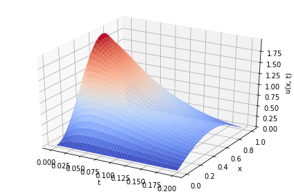
As this converges within nice numbers, the plot of the solution has the expected shape

Addendum: Crank-Nicolson

C-N is now the implicit trapezoidal method $$ U^{j+1}=U^j+\frac{Δt}2·(F(U^j)+F(U^{j+1})) $$ The linearization here is $$\begin{align} U^{j+1}+ΔU^{j+1}&=U^j+\frac{Δt}2\Bigl(F(U^j)+F(U^{j+1})+F'(U^{j+1})ΔU^{j+1}\Bigr)\\~\\ J·ΔU^{j+1}&=(I-γΔt·F'(U^{j+1}))·ΔU^{j+1}=U^j+γΔt·\Bigl(F(U^j)+F(U^{j+1})\Bigr)-U^{j+1} \end{align}$$ with $γ=\frac12$. Combine the terms in $U^j$ as they stay constant over the inner loop.

from scipy.sparse.linalg import spsolve, splu

for q in range(N):
    U[:, q+1] = U[:, q] + F(U[:, q])
    J = Jac(U[:, q+1], gamma=0.5)
    J_lu = splu(J)
    R = U[:, q] + 0.5*F(U[:, q+1])
    for p in range(4):
        #J = Jac(U[:, q+1])
        f = U[:, q+1] - 0.5*F(U[:, q+1]) - R
        U[:, q+1] -= J_lu.solve(f)
        print(q,p,max(abs(f)), max(abs(U[:,q+1])))

This works fine as well.