Numerical solution of an advection equation, $\frac{\partial P}{\partial t}+\frac{\partial}{\partial x}\left(P^{5/3}\right)=0$, with finite volume

Question

I was trying to solve the following equation numerically, $$\frac{\partial P}{\partial t}+\frac{\partial}{\partial x}\left(P^{5/3}\right)=0$$ I adopted the Godunov approach for discretising the equation numerically, $$\frac{P_{i}^{n+1}-P_{i}^{n}}{\Delta t}=-\frac{\mathcal{F}_{i+\frac{1}{2}}^{n}-\mathcal{F}_{i-\frac{1}{2}}^{n}}{x_{i+\frac{1}{2}}-x_{i-\frac{1}{2}}}$$ where $\mathcal{F}$ represents the numerical flux.

Following first order upwind scheme, I approximated the flux as, $$\mathcal{F}_{i+\frac{1}{2}}^{n}=\begin{cases} P_{i}^{5/3} & \text{if $P_{i}^{2/3}>0$}\\ P_{i+1}^{5/3} & \text{if $P_{i}^{2/3}<0$} \end{cases}. $$ However, with such a discretization, I am getting oscillations in the numerical solution. I am not sure if the discretization is correct. I will be grateful if someone can help me in this regard.

Answer 1

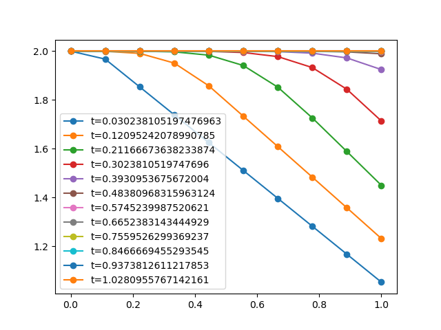
Your discretization with the upwind scheme looks correct.

One reason why you get oscillations might be that you are choosing an incorrect time step. Another one is if you have some complicated and not well-behaved boundary/initial conditions, some instabilities might arise if you don't handle them properly.

To compute a fair time step, that satisfies the Courant-Friedrichs-Lewy necessary stability condition, you can just take the maximum of the flow speed in your domain. Don't worry too much about how to compute the speed on the cell boundaries (fractional $i$), just take a fair value... The maximum of $P^{2/3}$ on the cell centers will be just fine. It is also a good practice to apply a safety factor $c \in ]0,1[$ to the $\Delta t$ you obtain in such a way, like

$$\Delta t = c 3/5 \Delta x / P^{2/3}$$

I implemented your scheme on your equation for a trivial set of boundary conditions ($P=2$) and initial conditions ($P=2$ on the left boundary, and drops linearly reaching value $P=1$ on the right boundary), and the solution I get looks well behaved:

import matplotlib.pyplot as plt
import numpy as np

#%% Settings
# Physical mesh points (you have to sum 1 left ghost cell)
Nx = 10
xStart = 0.
xEnd = 1.
tEnd = 1.

# Grid
x = np.linspace(xStart, xEnd, Nx)

# Initial condition
ic = np.linspace(2., 1., Nx)
# Boundary condition
bc = 2.

# Safety factor
Ccfl = 0.8

#%% Functions
def godunov(P, F, x, dt):
    return P[1:] - dt * (F[1:] - F[:-1]) / (x[1:] - x[:-1])

def flux(P):
    return P**(5/3)

#%% Solution
P = ic.copy()

Ps = []; ts = []
t = 0.
while t < tEnd:
    dt = Ccfl*3/5 * (xEnd - xStart)/Nx / max(P)**(2/3)
    F = flux(P)
    P = np.append([bc], godunov(P, F, x, dt))
    t += dt
    # Save results
    Ps.append(P)
    ts.append(t)

#%% Print results
fig, ax = plt.subplots()
for tt, t in enumerate(ts):
    if tt%3 == 0:
        ax.plot(x, Ps[tt], 'o-', label = f"t={t}")
        ax.legend()