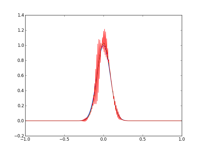
Quiet a lot of insight can be gained form experience, I was just wondering if anybody has seen something similar to this before. The plot shows the initial condition (green) for the advection-diffusion equation, then the solution at iteration 200 (blue) and then again at iteration 400 (red).

The solution of the advection-diffusion equation blows up after a few iterations. The Péclet number $\mu\approx0.07$, and the CFL condition is satisfied, $C\approx 0.0015$, so the equations should be stable. I anticipate I have a bug in the numerical code.
Background. The discretisation is central difference for both advection and diffusion terms. I believe this is first order of advection and second order for diffusion. I have implemented this using a finite-volume approach (for the first time) in which the coefficients (velocity and diffusion coefficient) values at the cell faces is found by linear interpolation from the cell averages. I apply Robin boundary condition on the left and right surfaces and set the flux at the boundaries to zero.
How do you debug your numerical code? Has anybody scene something like this before, where would be a good place to starting looking?
Update
- Here is my personal "lab book" style notes on implementing a finite volume method for the advection-diffusion equation, http://danieljfarrell.github.io/FVM/
- The Python source code is available here, http://github.com/danieljfarrell/FVM.git
Update
The solution couldn't be more simple! I just made a sign error on the diffusion term. It's strange, I'm sure it I had not of posted this I would not have found the error! If someone wants to share tips on how they debug their numerical code I am still interested. I don't have a method, it's a bit hit and miss, I keep on trying stuff to get clues, but this process can take weeks (sometimes).
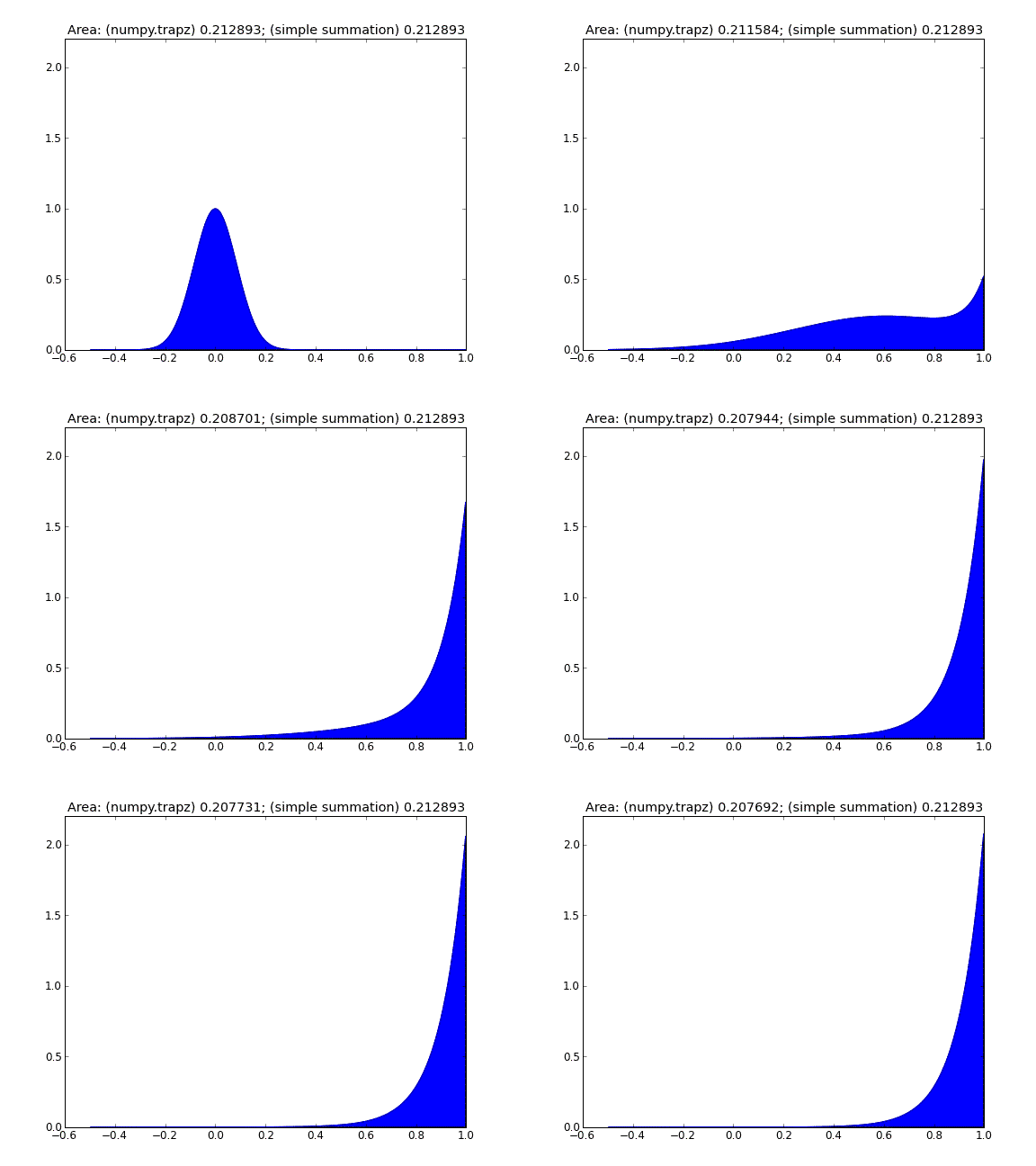
Proof it works (N.B. that with the finite-volume method all you need to do to calculate the area is a summation of width $\times$ height for all the cells, if you use an integration method such as numpy.trapz your results include the numerical error of the trapezium method). What is happening here? There is a constant velocity and diffusion coefficients but with closed boundary conditions. Therefore at the boundary we see the equilibrium between the velocity field pushing to the right and the diffusion push to the left.
