Amplitude of discrete Fourier transform of Gaussian is incorrect

Question

I am trying to understand why the amplitude of the FFT (computed with numpy) of a Gaussian differs from its analytic solution.

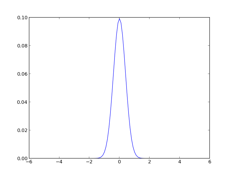
The $\mathcal{F}\{e^{-\pi t^2}\} = e^{-\pi f^2}$. However if I calculate it with the FFT function in numpy the resulting Gaussian's amplitude is not 1?

I have already done the following:

• I do divide the fft result by the number of samples (normalize).
• I have even tried shifting the Gaussian so that its first sample is its height. This corrects the sinusoidal behaviour, and removes the maginary part, but does not improve the amplitude result (same as absolute value of unshifted case). I will however be taking the absolute value in any case.

Here is the code:

def test_gauss_1D(self,a,f_c,delta_f):
   delta_t = 1.0/(2.0*f_c)
   N = int(np.ceil(1/(delta_f*delta_t)))+1
   if (N % 2) == 0:
      N = N + 1

   t = np.linspace(-(N-1)/2*delta_t,(N-1)/2*delta_t,N)
   f = np.linspace(-1/(2*delta_t),1/(2*delta_t),N)

   x_t = np.exp(-np.pi*t**2)

   #x_t = np.roll(x_t,-1*(N-1)/2)

   #x_t = 1/(np.sqrt(2*np.pi)*a)*np.exp(-t**2/(2*a**2))

   #print "std = ", 1/(4*a**2*np.pi**2)
   #print "ampl =", np.sqrt(2*np.pi)*a

   plt.plot(t,x_t)
   plt.show()

   #x_f = np.fft.fft(x_t)/N
   #print "N = ",N
   x_f = np.fft.fft(x_t)/N

   x_f = np.roll(x_f,1*(N-1)/2)

   plt.plot(f,np.absolute(f))
   plt.show()

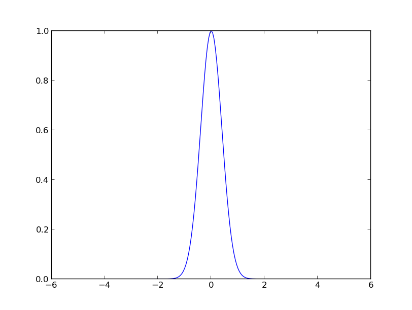
Here are the images:

As you can see the amplitude is incorrect in the second image (should be one).

Why is this?

Answer 1

The normalization needs to include the sampling frequency. Multiple your x_f by delta_t and you should be all set.

Answer 2

I think you have used an incorrect normalisation: the factor of 1/N is the result of applying both the transform and the inverse transform. For just the forward normalisation you therefore want 1/(sqrt(N)). When I run your code with this normalisation, I see a peak of sqrt(2), so the correct normalisation is therefore 1/(sqrt(2*N)).

I suspect that the final factor of two comes from the exact definition of N, and whether or not positive and negative frequencies should count twice. In any case, I can't seem to find it on the numpy documentation page: http://docs.scipy.org/doc/numpy/reference/routines.fft.html