Interpolation by Solving a Minimization Problem (Optimization)

Question

I will try to give the motivation behind this problem and later the math formality.
Given a grayscale image (1 Channel - $M \times N$ Matrix).
Someone marks some pixels as anchors.
Now, you need to interpolate the other pixels (Which are not anchors) by minimizing a given cost function s.t. the end result is an image which has the original image values at the anchors and interpolated values else were s.t. it minimizes the cost function.

Given an $M\times N$ matrix (A 1 channel image for that matter) $ I $.

A subset of the elements (Pixels) in the matrix are marked as a reference and their location is a group marked as $ S $.

The optimization cost function is given by:

$$ E = \arg \min_{E} \sum_{\mathbf{r}} \left( E(\mathbf{r}) - \sum_{\mathbf{s} \in N(\mathbf{r})} {w}_{\mathbf{rs}} E(\mathbf{s}) \right)^2, \text{ s.t. } \forall p \in S \; E(\mathbf{p}) = I(\mathbf{p})\,, $$

where a bold letter $ \mathbf{p}, \mathbf{r}, \mathbf{s} $ means an element (Pixel) location.

The group $ N(r) $ is the neighborhood of $ \mathbf{r} $, which is size $ k $ namely, a $ k $ by $ k $ rectangle where $ \mathbf{r} $ is in the middle.

The weights $ {w}_{\mathbf{rs}} $ are defined as following:

$$ {w}_{\mathbf{rs}} \propto \exp\left(-\frac{(I(\mathbf{r}) - I(\mathbf{s}))^2}{2\sigma^2_r} \right )\ \ \text{ s.t. } \sum_{\mathbf{s} \in N(\mathbf{r})} w_{\mathbf{rs}} = 1\,. $$

Namely, the weights are normalized to 1 within the neighborhood. The variance is calculated on the matrix $ I $ in the neighborhood (You can assume it is given).

So the problem is to find a matrix $ E $ which is equal to $ I $ on all reference points and interpolates other places by bringing the cost function to the minimum.

It looks like a weighted least squares per neighborhood, yet I couldn't formalize it in a way that can be easily calculated and solved in e.g. MATLAB.

Answer 1

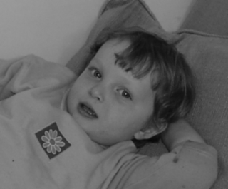
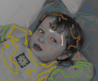
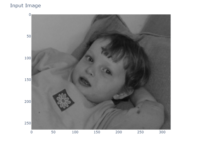
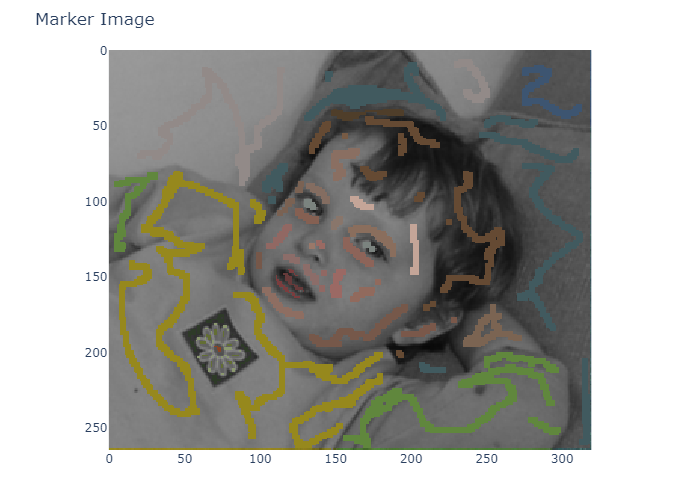
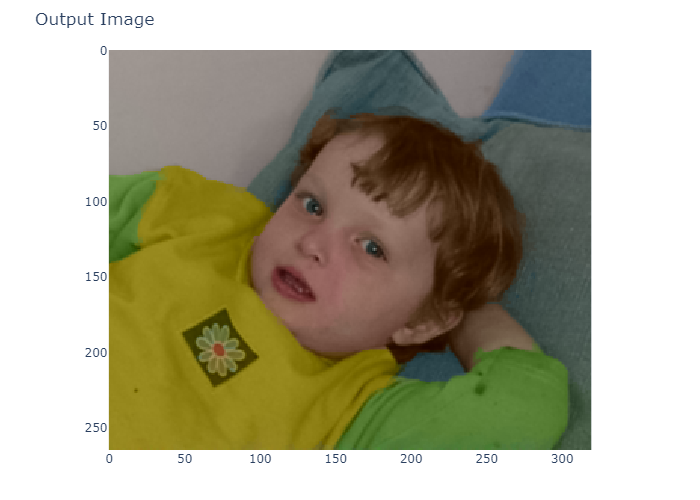
This is the classic colorization using optimization problem.

Optimization and Linear Algebra

To see how this can be expressed as a linear system, it's helpful to use a slightly different notation (and a slightly different objective function). Think of your image as graph $G$ with a node for each pixel in the image. There is an edge $(i,j)$ between two pixels $i$ and $j$, if these pixels are neighbors in the image.

Let $x_i$ be the intensity of pixel $i$, then you can write the problem as

$ \begin{array}{ll} \underset{x}{\mathrm{minimize}} & \frac{1}{2} \sum_{(i,j) \in E} w_{ij} (x_i - x_j)^2 \\ \mathrm{subject\ to} & x_i = d_i, i \in S. \end{array} $

For each edge in the graph we have weights denoted by $w_{ij} = w_{ji}$. Given this weighted graph $G(V, E, w)$ we can define the adjacency matrix $A$ by

$ A_{ij} = \begin{cases} w_{ij} & \text{if}\ (i,j) \in E\\ 0 & \text{otherwise} \end{cases} $

The degree matrix of a weighted graph is a diagonal matrix $D$ such that

$ D_{ii} = \sum_{j} A_{ij}$

The Laplacian matrix of a weighted graph is defined as $L = D - A$. With this definition of the Laplacian we can see that

$ x^T L x = \sum_{(i,j) \in E} w_{ij} (x_i - x_j)^2$

Thus we can rewrite the above problem in matrix form as:

$\begin{array}{ll} \underset{x}{\mathrm{minimize}} & \frac{1}{2} x^T L x \\ \mathrm{subject\ to} & x_m = d\\ \end{array} $

Here $L$ is the Laplacian matrix for the image, $x_m$ is the set of unknowns corresponding to marked pixels, and $d$ is the vector of annotated values (anchors).

Let $P$ be a permutation matrix (Hence $\boldsymbol{P}^{T} \boldsymbol{P} = \boldsymbol{P} \boldsymbol{P}^{T} = \boldsymbol{I}$) that orders $x$ so that the marked and unmarked unknowns are grouped such that

$ Px = \begin{bmatrix} x_m \\ x_u \end{bmatrix}$

Then we have that

$ \frac{1}{2} x^T L x = \frac{1}{2} x^T P^T (PLP^T) Px = \frac{1}{2} \begin{bmatrix} x_m^T & x_u^T \end{bmatrix} \begin{bmatrix} L_m & R^T \\ R & L_u \end{bmatrix} \begin{bmatrix} x_m \\ x_u \end{bmatrix}$

Here we have that $L_u = L_u^T \succ 0$. Since the values of the variables $x_m$ are fixed ($x_m = d$) we need only optimize over the variables $x_u$. Thus we can solve the unconstrained problem

$ \underset{x_u}{\mathrm{minimize}}\ F(x_u) = \frac{1}{2} x_u^T L_u x_u + x_m^T R^T x_u$

Since $L_u \succ 0$, the unique minimizer $x_u^\star$ is characterized by $\nabla F(x_u^\star) = 0$. We have that $\nabla F(x_u) = L_u x_u + R x_m$. Thus we need only solve the linear symmetric positive-definite system

$L_u x_u = -Rd$

You can solve this with a direct method (i.e. \ in MATLAB or conjugate gradient). For a class in grad school I implemented PCG in CUDA on a graphics card to color a 1050 x 3360 image which corresponded to a linear systems with 2.1 million unknowns. It took 230s on two Quadro FX 5600 GPUs to solve the system.

Sample MATLAB code

Below is sample MATLAB code which computes a colorization using the above images

original = double(imread('example.bmp'))/255;
marked   = double(imread('example_marked.bmp'))/255;

annotate_thresh = 0.25; % may need to be adjusted
colorim = sum(abs(original - marked), 3) > annotate_thresh;
colorim = double(colorim);
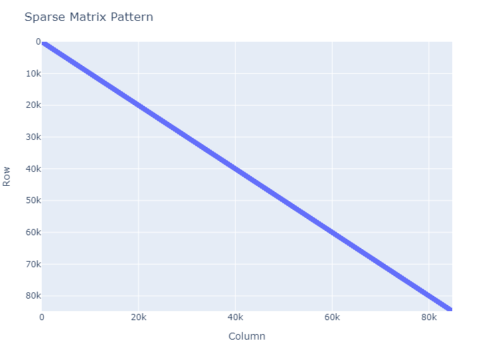
spy(colorim);
anchorind = find(colorim);

[m,n,p] = size(marked);
assert(p == 3);
N = m*n;

% convert from RGB to NTSC using the matrix T
T = [1.0 0.956 0.621; 1.0 -0.272 -0.647; 1.0 -1.106 1.703];
yiq = reshape(marked(:), N, 3)/T';
yiq = reshape(yiq, m, n, 3);
chromi = yiq(:,:,2);
chromq = yiq(:,:,3);
% Get grayscale value from original image
yiq = reshape(original(:), N, 3)/T';
yiq = reshape(yiq, m, n, 3);
gray = yiq(:,:,1);

% Get anchors from the I and Q color components
anchor(:,1) = chromi(anchorind);
anchor(:,2) = chromq(anchorind);

edges=[(1:N)' ((1:N)+1)'];        %add downard edge between node i with node i+1
edges=[edges; (1:N)' (1:N)'+m];   %add leftward edge between node i and i+m
% exclude edges which link to nodes outside the domain
excluded=edges(:,1)>N | edges(:,1)<1 | edges(:,2)>N |edges(:,2)<1; 
edges(excluded, :) = [];
% remove edge from bottom of column to top of next column
edges((m:m:(m-1)*n)',:)=[]; 

beta = 200;
EPSILON = 1e-5;

% calculate edge weights
graydistance = abs(gray(edges(:,1)) - gray(edges(:,2)));
ming = min(graydistance);  % it's helpful to normalize distances
maxg = max(graydistance);
graydistance = (graydistance - ming)./(maxg - ming);
weights=exp(-(beta*graydistance)) + EPSILON;

%Build sparse weighted adjacency matrix
W=sparse([edges(:,1);edges(:,2)],[edges(:,2);edges(:,1)], ...
    [weights;weights],N,N);
% Build Degree matrix
D = diag(sum(W));
% Build Laplacian
L=D-W;

mark = anchorind;
rest = 1:n*m;
rest(mark) = [];
rest = rest';
% Extract the portion of the Lapalcian matrices
Lu = L(rest, rest);
R  = L(rest, mark);
recover = zeros(m, n, 3);
recover(:,:,1) = gray;
xchannel = zeros(m*n,1);
for i=1:2
    d  = anchor(:,i);
    xrest = -Lu\(R*d);
    xchannel(rest) = xrest;
    xchannel(mark) = d;
    recover(:,:,i+1) = reshape(xchannel, m, n);
end
% Convert from YIQ back to RGB using T matrix
recover = reshape(recover, m*n, 3);
recover = recover*T';
% Keep RGB values within [0,1]
recover = min(max(0, recover), 1);
final   = reshape(recover, m, n, 3);

figure(1);
image(final);

The output is the image below

Why a different objective function

I choose a different objective function than the one stated in your problem. There are several reasons for this:

1. The quantity $w_{ij} (x_i - x_j)^2$ has a clear interpretation in the objective. You pay a weighted penalty based on the square of the difference between two adjacent pixels.
2. Using the definition of the Laplacian matrix $L$ it's easy to go from this objective function to the matrix equation $x^T L x$.
3. Using the definition of $L = A^T C A$ (where $A$ is the edge-node adjacency matrix and $C$ is a diagonal matrix containing the edge weights) it's easy to see that the Laplacian is positive semi-definite. If we add a small bit of regularization to make it positive definite, we can solve systems with $L$ via a Cholesky factorization or preconditioned conjugate gradient.
4. It's possible to do everything with the objective function you defined above. It's just more difficult to figure out how to translate it into a matrix equation.

Note the idea of using this different objective function is not my own. I found it in a paper by Leo Grady on Random Walks for Image Segmentation (See presentation Random Walks for Image Segmentation).

Working with large images

An image with $m$ rows and $n$ columns will yield a matrix $L$ of size $mn \times mn$. The number of nonzeros in $L$ is related to the size of the neighborhood around a pixel. In the code above, each pixel can have up to four neighbors: up, down, left, right. So the number of nonzeros in $L$ is bounded by $5mn$. Holding $L$ in memory is equivalent to having a small number of copies of the image in memory.

If you want to work with large images, you probably want to use some sort of iterative method. Iterative methods don't require you to form $L$ directly, but rather compute matrix-vector products. That is given a vector $x$ compute a vector $y$ such that $y=Lx$. As I mentioned above, I used preconditioned conjugate gradient, with diagonal preconditioning, on multiple graphics cards to solve this problem. This worked OK, but was still fairly slow on large images. To work with large images efficiently you may need to come up with a better preconditioner. There's been some research on this, for example see Richard Szeliski's paper on "Locally Adapted Hierarchical Basis Preconditioning". I think others have also investigated using multigrid methods to solve this problem.

Answer 2

Using few tricks the equation can be transformed into classic Quadratic Programming problem:

$$ E = \arg \min_{E} \sum_{\mathbf{r}} \left( E(\mathbf{r}) - \sum_{\mathbf{s} \in N(\mathbf{r})} {w}_{\mathbf{rs}} E(\mathbf{s}) \right)^2 $$

Defining $ \boldsymbol{e} = vec \left ( E \right ) $, Namely vectorizing the matrix, and defining a matrix $ A $ defined the proper usage of the weights $ {w}_{\mathbf{rs}} $, Namely put them in the correct entry at each row per pixel the above could be rewritten as:

$$ \hat{\mathbf{e}} = \arg \min_{\mathbf{e}} {\left ( \mathbf{e} - A\mathbf{e} \right ) }^{T} \left ( \mathbf{e} - A\mathbf{e} \right ) = \arg \min_{\mathbf{e}} {\left( \left ( I - A \right ) \mathbf{e} \right )}^{T} \left( \left ( I - A \right ) \mathbf{e} \right ) $$

Defining $ B = I - A $ yields:

$$ \hat{\mathbf{e}} = \arg \min_{\mathbf{e}} {\left( \left ( I - A \right ) \mathbf{e} \right )}^{T} \left( \left ( I - A \right ) \mathbf{e} \right ) = \arg \min_{\mathbf{e}} {\mathbf{e}}^{T} {B}^{T} B \mathbf{e} $$

Defining $ L = {B}^{T} B $ , namely $ L $, is a Symmetric Positive Definite Matrix yields:

$$ \hat{\mathbf{e}} = \arg \min_{\mathbf{e}} {\mathbf{e}}^{T} L \mathbf{e} $$

Adding the equality constraints using $ C \mathbf{e} = \mathbf{t} $ where $ \mathbf{t} $ is vectorization of all "Reference Pixels"

All in all this yields a Classic Quadratic Programming problem given by:

$$ \hat{\mathbf{e}} = \arg \min_{\mathbf{e}} {\mathbf{e}}^{T} L \mathbf{e}, \; s.t. \; C \mathbf{e} = \mathbf{t} $$

Few notes:

1. The matrix $ L $ is Symmetric and Positive Definite matrix and usually sparse (Assuming "Small Neighborhood").
2. The matrix $ L $ was built by the Matrix $ I - A $ which each row of it was normalized to be zero (Each row of $ A $ is normalized to 1).

Now two things are needed:

1. Optimized fast algorithm to solve this problem utilizing its properties.
2. Assuming the image is large, are there methods to solve this problem by blocks to avoid memory limits?

Answer 3

I implemented the algorithm in Julia.
The motivation is being able to control better the memory allocations and hence get faster results.

The formulation I used is:

$$\begin{align} \arg \min_{\boldsymbol{x}} \quad & \frac{1}{2} \boldsymbol{x}^{T} \boldsymbol{L} \boldsymbol{x} \\ \text{subject to} \quad & \begin{aligned} {x}_{i} & = {d}_{i} \; \forall i \in \mathcal{V} \\ \end{aligned} \end{align}$$

Where $\mathcal{V}$ is the set of pixel indices which have a reference value.

The trick with the Permutation Matrix allows to order the pixels:

$$ \begin{bmatrix} \boldsymbol{x}_{\mathcal{U}} \\ \boldsymbol{x}_{\mathcal{V}} \end{bmatrix} = \boldsymbol{P} \boldsymbol{x} $$

Since for any Permutation Matrix $ \boldsymbol{P} \boldsymbol{P}^{T} = \boldsymbol{P}^{T} \boldsymbol{P} = \boldsymbol{I} $ then:

$$ \boldsymbol{x}^{T} \boldsymbol{L} \boldsymbol{x} = \boldsymbol{x}^{T} \boldsymbol{P}^{T} \left( \boldsymbol{P} \boldsymbol{L} \boldsymbol{P}^{T} \right) \boldsymbol{P} \boldsymbol{x} = \begin{bmatrix} \boldsymbol{x}_{\mathcal{U}} & \boldsymbol{x}_{\mathcal{V}} \end{bmatrix} \begin{bmatrix} \boldsymbol{L}_{\mathcal{U}} & \boldsymbol{R} \\ \boldsymbol{R} & \boldsymbol{L}_{\mathcal{V}} \end{bmatrix} \begin{bmatrix} \boldsymbol{x}_{\mathcal{U}} \\ \boldsymbol{x}_{\mathcal{V}} \end{bmatrix} $$

Since the permutation matrix means no interaction between pixels (As opposed to equality with general matrix) then one can choose the subset, which interacts with $\boldsymbol{x}_{\mathcal{U}}$, to solve which becomes:

$$\begin{align} \arg \min_{\boldsymbol{x}_{\mathcal{U}}} \quad & \frac{1}{2} \boldsymbol{x}_{\mathcal{U}}^{T} \boldsymbol{L}_{\mathcal{U}} \boldsymbol{x}_{\mathcal{U}} + \frac{1}{2} \boldsymbol{x}_{\mathcal{v}}^{T} \boldsymbol{R} \boldsymbol{x}_{\mathcal{U}} \\ \text{subject to} \quad & \begin{aligned} {x}_{i} & = {d}_{i} \; \forall i \in \mathcal{V} \\ \end{aligned} \end{align}$$

Where $ \boldsymbol{x}_{\mathcal{v}} = \boldsymbol{d} $.
Hence the problem becomes constraint free:

$$ \arg \min_{\boldsymbol{x}_{\mathcal{U}}} \frac{1}{2} \boldsymbol{x}_{\mathcal{U}}^{T} \boldsymbol{L}_{\mathcal{U}} \boldsymbol{x}_{\mathcal{U}} + \frac{1}{2} \boldsymbol{x}_{\mathcal{v}}^{T} \boldsymbol{R} \boldsymbol{x}_{\mathcal{U}} $$

This is a strictly convex problem and the gradient vanishes at:

$$ \boldsymbol{L}_{\mathcal{U}} \hat{\boldsymbol{x}}_{\mathcal{U}} = - \boldsymbol{R} \boldsymbol{x}_{\mathcal{V}} $$

Which can be solved either directly or using Conjugate Gradient.
The direct solver should take advantage of the fast the matrix is Positive Definite. Since the same matrix is used for 2 image channels, it is better to apply the symbolic factorization once.

The Graph Laplacian Matrix, $\boldsymbol{L} = \boldsymbol{D} - \boldsymbol{W}$, is the result of generating the Affinity / Similarity / Adjacency Matrix and the Degree Matrix.

The weights are calculated by:

$$ {W}_{i, j} \propto \exp\left(- \beta \left| I \left( i \right) - I \left( j \right) \right| \right ) + \epsilon $$

One could choose many more options for affinity / similarity measure.
The added $\epsilon$ assists with numerical difficulties.

The weights should also be normalized.
One could normalize the affinity matrix such that each row has a sum of one as suggested in the question.
The code actually normalizes the distances between the pixels into the range $\left[ 0, 1 \right]$ and then applies the affinity transformation as written above.

I implemented a generalized function to build the weights matrix $\boldsymbol{W}$. It basically loops over the pixels and applies a user defined function which has the input of the 2 values, the indices and the neighborhood shift indices.
This way I could try affinity of 3x3 yet it seems that 4 Connectivity gets better results.
Pay attention not to calculate the self weight (Pixel to itself).

Remarks:

• The derivation of the objectives follows the solution by @codehippo.
  I rewrote it in a manner clearer to me.
• The objective is similar to Normal Cuts objective in Graphs.
• The derivation is equivalent to my Wiki post in case the affinity matrix is indeed normalized to have rows of sum 1. Then the same trick to avoid the equality can be employed.
• Using Preconditioned CG will be much faster for larger cases.

---

The code is available on my StackExchange Computational Science GitHub Repository (Look at the ComputationalScience\Q11387 folder).