I am not sure if I understand the question completely, but I will try to answer.
In brackets you have an operator in an infinite dimensional space, although the first one is a derivative and the second one a multiplicative operator. Under some representations they would admit an (infinite) matrix form. And, when you approximate the solution you would end up with a finite dimensional approximation, where the operators are represented by matrices.
As I mentioned in the answer you link to, Finite Differences would be the easiest approach, but no the only one. You could try with Finite Element Methods, but the second term makes me wonder. In the case of Finite Differences, you would end up with similar matrices, but now you have a problem that would not appear in 1D, ordering the cells. In 1D, they are "naturally" ordered from left to right. But in 2D you would need to decide how. The most straightforward would be to consider that you have a rectangular grid and you number by rows first and then by columns (or the opposite way). Nothing says that you cannot have a different order, but it is easier this way. You might found references 1 and 2 useful.
Now, taking as a base my code from the previous answer, let's consider the quantum harmonic oscillator first (in normalized units)
$$\left[-\frac{1}{2}\nabla^2 + \frac{1}{2}(x^2 + y^2)\right] \psi = E \psi$$
that has as eigenvalues $E_{m,n} =[(m + n) + 1]$ where $m, n$ are non-negative integers. And, let's assume that we have equal partitions in $x$ and $y$, in number and size $N$.
The Laplace operator would have 5 diagonals, below an example for $N=3$. Three diagonals are consecutive, since the cells are contiguous, and the other one have a spacing of $N$ from the center (as cells in the grid).
$$T = -\frac{1}{2 \Delta x}\begin{bmatrix}
-4 & 1 & 0 & 0 & 1 & 0 & 0 & 0 & 0\\
1 & -4 & 1 & 0 & 0 & 1 & 0 & 0 & 0\\
0 & 1 & -4 & 1 & 0 & 0 & 1 & 0 & 0\\
0 & 0 & 1 & -4 & 1 & 0 & 0 & 1 & 0\\
1 & 0 & 0 & 1 & -4 & 1 & 0 & 0 & 1\\
0 & 1 & 0 & 0 & 1 & -4 & 1 & 0 & 0\\
0 & 0 & 1 & 0 & 0 & 1 & -4 & 1 & 0\\
0 & 0 & 0 & 1 & 0 & 0 & 1 & -4 & 1\\
0 & 0 & 0 & 0 & 1 & 0 & 0 & 1 & -4
\end{bmatrix}$$
The other term is the multiplicative operator, that can be represented as a diagonal matrix with the values for $1/2(x^2 + y^2)$ in each cell, i.e.
$$U = \frac{1}{2}\begin{bmatrix}
x_0^2 + y_0^2 & 0 &\cdots &0\\
0 &x_1^2 + y_1^2 &\cdots &0\\
\vdots &\vdots &\ddots &\vdots\\
0 &0 &\cdots &x_{N^2}^2 + y_{N^2}^2
\end{bmatrix}$$
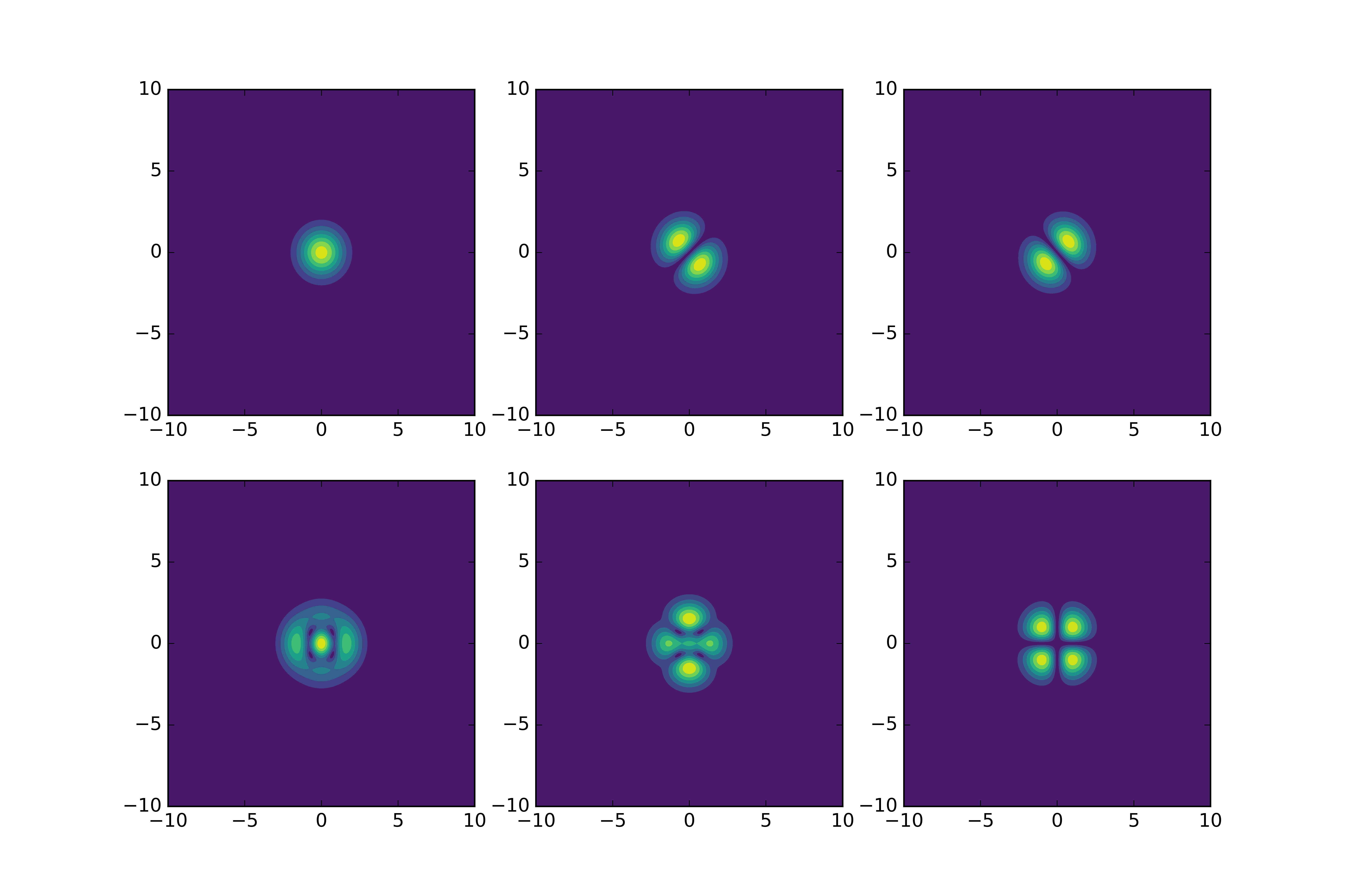
The code below solves this problem, with the first six eigenvalues being
[ 0.9999 1.9997 1.9997 2.9993 2.9993 2.9995]
that is close to the theoretical values [1.0, 2.0, 2.0, 3.0, 3.0, 3.0].
from __future__ import division
import numpy as np
from scipy.sparse import diags
from scipy.sparse.linalg import eigsh
import matplotlib.pyplot as plt

L = 20
N = 501
dx = L/(N - 1)
X, Y = np.mgrid[-L/2:L/2:1j*N,-L/2:L/2:1j*N]

T = -0.5*diags([-4., 1., 1., 1., 1.], [0,-1, 1, -N, N],
               shape=(N**2, N**2))/dx**2
U_vec = 0.5*(X**2 + Y**2)
U_vec.shape = N**2
U = diags([U_vec], [0])

H = T + U

vals, vecs = eigsh(H, which='SM')
order = np.argsort(vals)
vals = vals[order]
vecs = vecs[:, order]

#%%
print np.round(vals, 6)
plt.figure(figsize=(12, 8))
for k in range(6):
    plt.subplot(2, 3, k+1)
    vec = vecs[:, k]
    mag = np.sqrt(np.dot(vecs[:, k],vecs[:, k]))
    vec = vec/mag
    vec.shape = X.shape
    plt.contourf(X, Y, np.abs(vec), cmap="viridis")

plt.savefig("quantum_harmonic.png", dpi=600)
plt.show()

Now, if we add the other term we would have a new operator. I would show it for the first term in parenthesis. The derivative with respect to $x$ (and imaginary unite) can be represented as
$$D_x = \frac{i}{\Delta x}\begin{bmatrix}
0 & 1 &\cdots &0 &0\\
-1 &0 &\cdots &0 &0\\
\vdots &\vdots &\ddots &\vdots &\vdots\\
0 &0 &\cdots &0 &1\\
0 &0 &\cdots &-1 &0
\end{bmatrix}$$
and the multiplication by $y$ would be
$$Y = \begin{bmatrix}
y_0 & 0 &\cdots &0\\
0 &y_1 &\cdots &0\\
\vdots &\vdots &\ddots &\vdots\\
0 &0 &\cdots &y_{N^2}
\end{bmatrix}$$
The other term is similar, the $D_y$ would have two non-zero diagonals in the $N$ and $-N$ diagonals. The final matrix would be
$$H = T + 2U + YD_x - XD_y$$
I am using $2U$ because of the $1/2$ that I used before. The following code presents this approach
from __future__ import division
import numpy as np
from scipy.sparse import diags
from scipy.sparse.linalg import eigsh
import matplotlib.pyplot as plt

L = 20
N = 501
dx = L/(N - 1)
X, Y = np.mgrid[-L/2:L/2:1j*N,-L/2:L/2:1j*N]

T = -0.5*diags([-4., 1., 1., 1., 1.], [0,-1, 1, -N, N],
               shape=(N**2, N**2), dtype=np.complex)/dx**2
U_vec = X**2 + Y**2
U_vec.shape = N**2
DX = diags([-0.5j, 0.5j], [-1, 1], shape=(N**2, N**2), dtype=np.complex)/dx
DY = diags([-0.5j, 0.5j], [-N, N], shape=(N**2, N**2), dtype=np.complex)/dx
Xmat = diags([np.reshape(X, (N**2))], [0], dtype=np.complex)
Ymat = diags([np.reshape(Y, (N**2))], [0], dtype=np.complex)
U2 = np.dot(Ymat, DX) - np.dot(Xmat, DY)
U = diags([U_vec], [0]) +  U2

H = T + U

vals, vecs = eigsh(H, which='SM')
order = np.argsort(vals)
vals = vals[order]
vecs = vecs[:, order]

#%%
print np.round(vals, 6)
plt.figure(figsize=(12, 8))
for k in range(6):
    plt.subplot(2, 3, k+1)
    vec = vecs[:, k]
    mag = np.sqrt(np.dot(vecs[:, k],vecs[:, k]))
    vec = vec/mag
    vec.shape = X.shape
    plt.contourf(X, Y, np.abs(vec), cmap="viridis")


plt.savefig("eigenvectors.png", dpi=600)
plt.show()
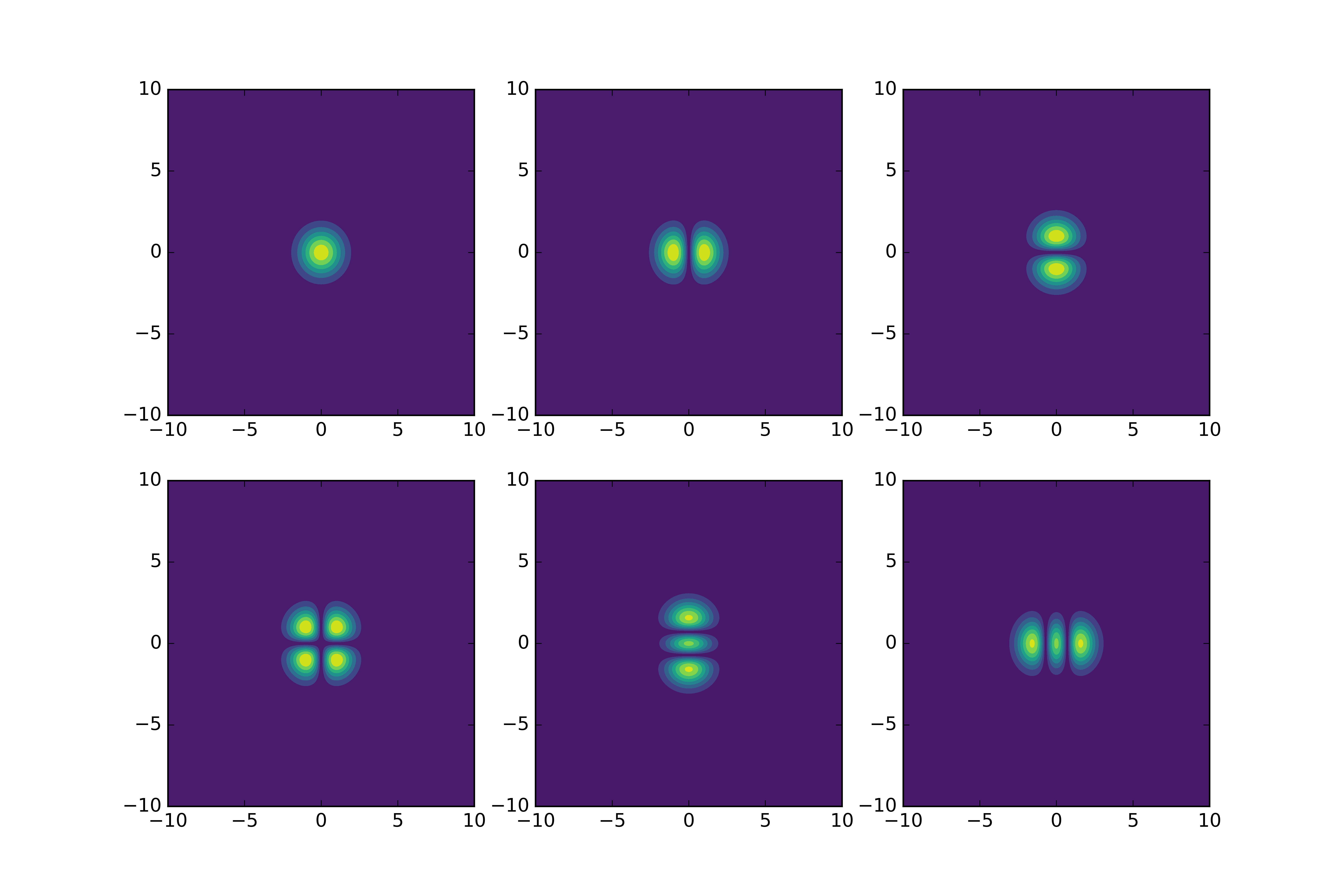
The eigenvalues are [ 1.000399 2.001196 2.001196 3.001993 3.002786 3.002786], that seem slightly perturbed over the harmonic oscillator... but I don't really know if they are correct or not. The eigenvectors are presented below, the first three make sense to me, but one more time, I don't know about the others.

Notes
- I am using second order finite differences, but you could pick other orders.
- The domain used in the codes is finite. That is one easy way of approaching the infinite domain, since outside that region the probability density is small enough. A better approach is to use special boundary conditions that mimics the infinite region outside.
- Even for the finite domain, it would be a better choice to have small cell in the center and bigger ones in the outside. This is because most of the "interesting" things would happen in the center, where the potential is smaller and hence the probability density higher.
- I am not considering boundary conditions in this case, although they are somehow implicitly taken into account. In general, you should consider those, specially if your domain is finite.
References
- Korsch, H. J., and M. Glück. "Computing quantum eigenvalues made easy." European journal of physics 23.4 (2002): 413.
- Garcia, Rafael, Alex Zozulya, and James Stickney. "MATLAB codes for teaching quantum physics: Part 1." arXiv preprint arXiv:0704.1622 (2007).

