Why the magnetisation shows abrupt behaviour for this 3D ising spin system

Question

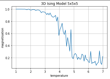
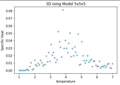
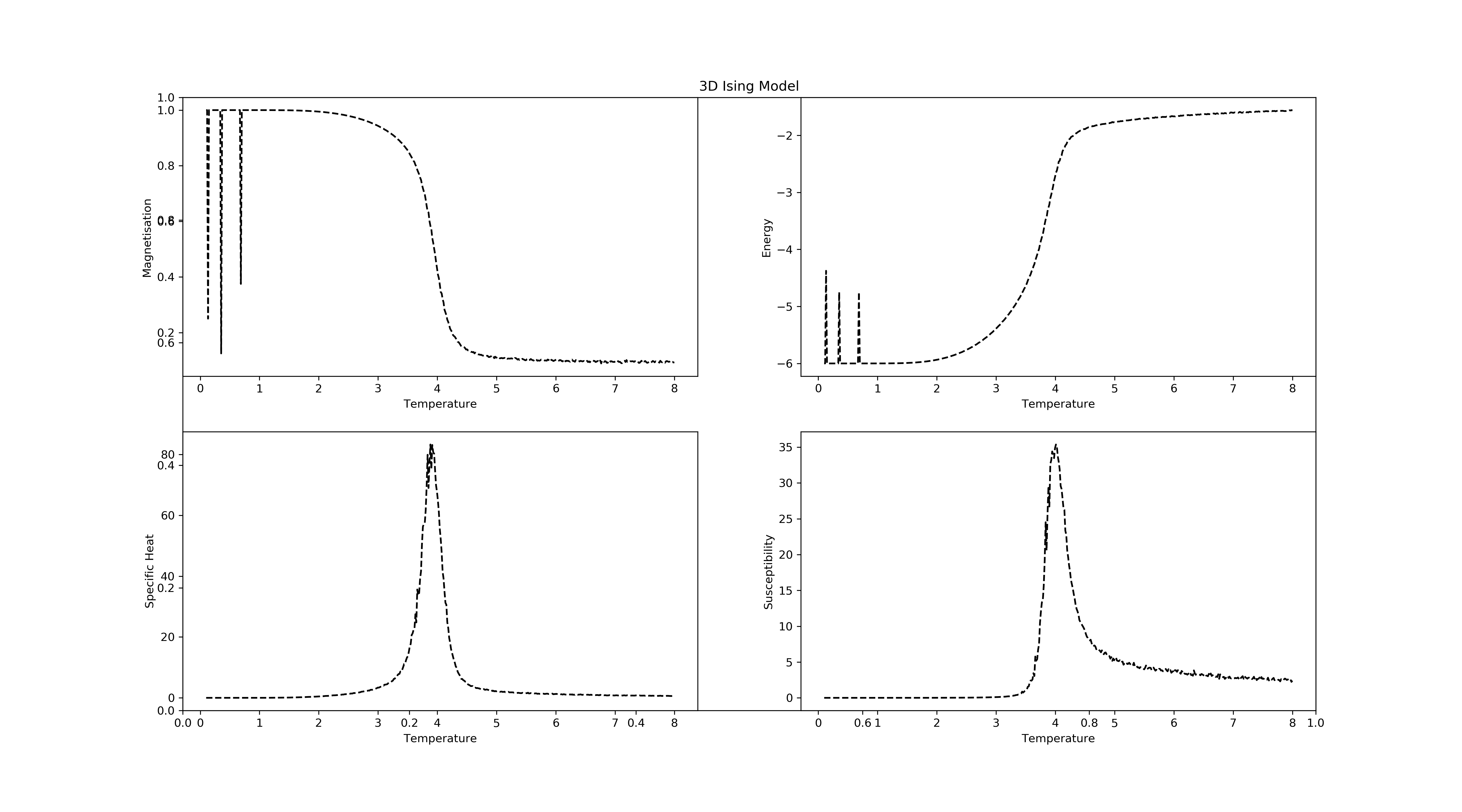
I am trying to simulate a 3D Ising spin system (+1 & -1) using Monte Carlo Metropolis Algorithm. I want to get different physical quantities from this simulation like magnetization, Average Energy, Susceptibility, Specific Heat. I have used exactly similar code for 2 dimension that gives perfect result but for 3D it fails. The magnetization curve is quite noisy. In spite of increasing trials it always shows sudden valleys. I have made all the required modifications for 3D but can't find out what is going wrong. The specific heat also does not show the discontinuity in the right manner.

The following code simulates for a 3d Ising spin system 5x5x5 with 1250 Monte Carlo steps (excluding 2000 steps to let the system reach equilibrium). Currently, it only calculates magnetization.Below is the plot I am currently getting from the code.

# cost            change in energy
# J               spin coupling constant, will be normalised
# spin_states     3D array, the lattice
# M               total magnetisation of the lattice
# m               magnetisation per spin { m = M / (N * N * N) }
# N               size of the lattice


from numpy.random import rand

import numpy as np     
import matplotlib.pyplot as plt    
import time     # for timing





def initialise(N):   
   ''' generates a random spin spin_statesuration for initial condition'''
   spin_states = np.random.choice([1, -1], size=(N, N,N))
   #spin_states=np.ones([N,N,N])
   return spin_states



def calcMag(spin_states):
   '''Magnetization of a given spin_statesuration'''
   mag = abs(np.sum(spin_states))
   return mag

def calcEnergy(spin_states):
   '''Energy of a given spin_statesuration'''
   energy = 0
   for i in range(len(spin_states)):
       for j in range(len(spin_states)):
           for k in range(len(spin_states)) :
               s = spin_states[i,j,k]
               energy += -s*find_neighbours(spin_states,N,i,j,k)
   return energy/8.

def find_neighbours(spin_states,N,x,y,z):
   left   =spin_states[x,(y-1)%N,z]
   right  =spin_states[x,(y+1)%N,z]
   top    =spin_states[(x-1)%N,y,z]
   bottom =spin_states[(x+1)%N,y,z]
   front  =spin_states[x,y,(z+1)%N]
   back   =spin_states[x,y,(z-1)%N]

   tot_spin=left+right+top+bottom+front+back 

   return (tot_spin)

def mcmove(spin_states, beta):
   '''Monte Carlo move using Metropolis algorithm '''
   x = np.random.randint(0, N)
   y = np.random.randint(0, N)
   z = np.random.randint(0, N)
   s = spin_states[x, y, z]

   cost = 2*s*find_neighbours(spin_states,N,x,y,z)
   if cost < 0:
       s *= -1
   elif rand() < np.exp(-cost*beta):
       s *= -1
   spin_states[x, y,z] = s
   return spin_states

nt      = 80         #  number of temperature points
N       = 5        #  size of the lattice, size x size
eqSteps = 2000       #  number of MC sweeps for equilibration
mcSteps = 1250       #  number of MC sweeps for calculation



spin_states = initialise(N)

m = calcMag(spin_states)
print ("m =", m)

#k = mcSteps * N * N * N


dataM = []

T       = np.linspace(1, 7, nt) 
E,M,C,X = np.zeros(nt), np.zeros(nt), np.zeros(nt), np.zeros(nt)
n1, n2  = 1.0/(mcSteps*N*N*N), 1.0/(mcSteps*mcSteps*N*N*N)
for tt in range(nt):
   E1 = M1 = E2 = M2 = 0
   spin_states = initialise(N)
   iT=1.0/T[tt]; iT2=iT*iT;   # inverse temperature for beta

   for i in range(eqSteps):         # equilibrate
       mcmove(spin_states, iT)           # Monte Carlo moves

   for i in range(mcSteps):
       mcmove(spin_states, iT)           
       Ene = calcEnergy(spin_states)     # calculate the energy
       Mag = calcMag(spin_states)        # calculate the magnetisation

       E1 = E1 + Ene
       M1 = M1 + Mag
       M2 = M2 + Mag*Mag 
       E2 = E2 + Ene*Ene

   E[tt] = n1*E1
   M[tt] = n1*M1
   C[tt] = (n1*E2 - n2*E1*E1)*iT2
   X[tt] = (n1*M2 - n2*M1*M1)*iT




print(M)    
plt.plot(T,M)
plt.xlabel('temperature')
plt.ylabel('magnetisation')
plt.title('3D Ising Model')
plt.grid(True)
plt.show()

plt.figure()
plt.plot(T,C,'+')

Please can anybody help me to find out what is going wrong? As far as I can think, the metropolis algorithm is really doing not much change. I have done the simulation for diff. lattice sizes with diff no. of steps. It never changes much from the initial value. I am new to simulation and this is my second simulation project. Any help will be much appreciated. Thank you in advance.

Answer 1

Your lattice consists of 5 x 5 x 5 = 125 spins, so your number of Montecarlo steps to reach equilibrium should be >> 125, because you randomly picking a site and flipping it, so random numbers should uniformly generated so that it will cover whole lattice. For much finer measurement of thermodynamic quantities, you should take more number of points between the temperature range and more number of Montecarlo steps >> 25.

So I modified your code a bit, instead of picking a site randomly and flipping, I swept through each site starting row and column wise.

def mcmove(spin_states, beta):
    '''Monte Carlo move using Metropolis algorithm '''
    for x in range(len(spin_states)):
        for y in range(len(spin_states)):
            for z in range(len(spin_states)):
                s = spin_states[x,y,z]
                cost = 2*s*find_neighbours(spin_states,N,x,y,z)
                if cost < 0:
                    s *= -1
                elif rand() < np.exp(-cost*beta):
                    s *= -1
                spin_states[x, y,z] = s
    return spin_states

I ran the simulations on a 16 x 16 x 16 lattice, temperature ranging from 0.1 - 8.0 with 500 points in-between, with 5000 steps to reach equilibrium and 5000 steps to take measurement (you can get similar results with less number of Montecarlo steps, say 100 + 100, since it will sweep through whole lattice). These are my results