3
$\begingroup$

I'd like to program a trajectory planner, let's say for a robot, and I can pass acceleration commands to the robot, the robot can move in one dimension. The outcome of the planner is now a vector with accelerations, for example 10 accelerations, and since I set the accelerations with a frequency of 2, this will be sufficient to steer the robot for the next 5 seconds.

The trajectory should be planned in a way that (a) minimizes jerk and (b) is as near at the desired velocity as possible. So I know what makes up my fitness function: sum over squared jerks and squared differences v, v_desired.

So I want to minimize jerk. I thought I search for a jerk profile (that is, jerk values at 10 discrete times, like 0.5, 1, ..., 5, to be consistent with the example above), integrate this twice so that I also have the speed profile, and apply my fitness function. The jerk profile is searched with a particle swarm optimizer. The nice thing is, 0 is already a good initialization for the profile.

Then I thought about approximating the jerk profile with a polynomial, and not to search for the profile directly, but for the polynomial parameters. This way, integration would be trivial, everything would be steady and smooth, and I could sample points at whatever times I'd like. At least I thought this was a good idea.

So my question is: Are polynomials a good tool for this? I can't believe that estimating e.g. 5 parameters (and evaluating the resulting polynomial at e.g. 30 positions) will yield better results than searching for 30 points (the jerk) directly. My experiments from the last hours shows that the curves very quickly start looking like waves, and that's not what you want for a trajectory, especially not for the velocity profile ...

Is my approach with "estimate function parameters rather than sample points" bad? Is a polynomial bad? Are there better functions, easily to extend in number of parameters and trivially to integrate?

I hope my question is understandable, if not, please complain and I will try being more specific.

UPDATE

The picture below shows the result of my first approach, with "optimizing" parameters for a 4th degree polynomial for jerk. This was integrated with the correct initial values for a, v and s in my one-dimensional world. The initial v was set to 5.0, v desired is 2.0, and initial acceleration was 2.0. I would expect the velocity to first increase (caused by the initial acceleration), and then decrease slowly to 2. At point number 10, you can see the "overshoot" of v and the wiggly behaviour mentioned in the first comment.
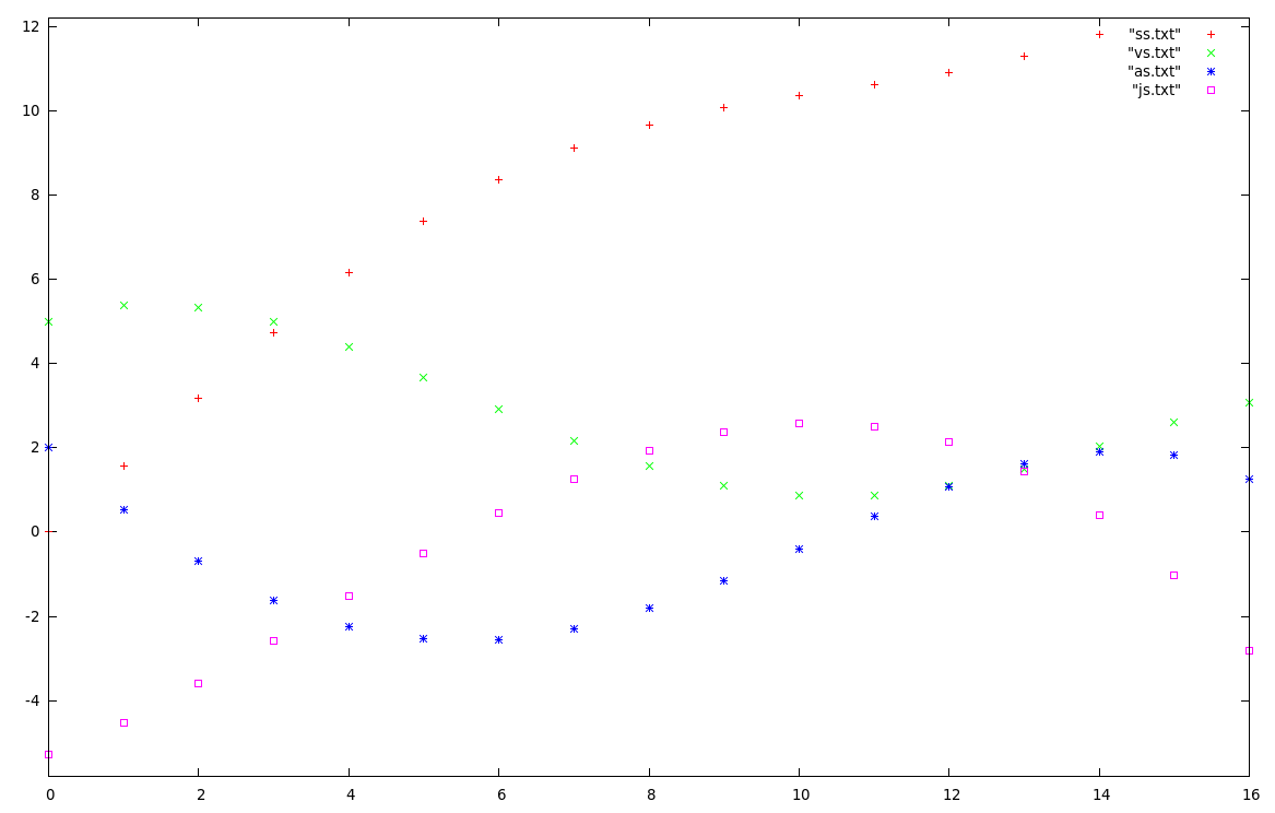
attempt at a trajectory

$\endgroup$
6
  • $\begingroup$ It might be more profitable to use piecewise polynomials instead of polynomials, since high-degree polynomials tend to wiggle rather wildly. You might want to look into using splines with the appropriate sort of continuity; maybe $C^4$ quintic splines? $\endgroup$
    – J. M.
    Commented May 19, 2013 at 14:54
  • $\begingroup$ Wiggly – exactly this is the word I should have found when formulating my question. Regarding splines: So it should be possible to say "my acceleration function consists of 5 splines" and I then search for good parameters? I know splines only for interpolation. $\endgroup$
    – user4344
    Commented May 19, 2013 at 14:57
  • $\begingroup$ If it's not too much trouble, can you post a plot of the points you were using to build a path? I see that you do not yet have sufficient rep, so at least post a link to the picture, and someone can edit your post to embed the picture. $\endgroup$
    – J. M.
    Commented May 19, 2013 at 15:00
  • $\begingroup$ "my acceleration function consists of 5 splines" - more like "a spline with $n$ pieces", with each piece being a suitable low-degree polynomial. I suggested looking for something with $C^4$ continuity, since it seems you want the jerk to be continuous as well; quintic splines can fit the bill. (Cubic splines only have $C^2$ continuity, so not suitable for you.) $\endgroup$
    – J. M.
    Commented May 19, 2013 at 15:02
  • $\begingroup$ Since I integrate, will cubic not be sufficient? I understand your comment like you care that I cannot differentiate cubic splines often enough ... $\endgroup$
    – user4344
    Commented May 19, 2013 at 15:25

2 Answers 2

2
$\begingroup$

Ok, I experimented a lot today and using splines definitely looks promising. Although a little bit more computational effort to setup the splines (inversion of a matrix and so on, but I used Eigen3 for that), integration is rather trivial. With the polynomial representation, I can do a lot analytically, for example, the costs for deviation in velocity will become a difference of polynomials (one of a piecewise aka. spline and one of zeroth degree, constant), and it's exactly one step to get the costs, no need to draw samples at discrete points and sum them up. Don't know if I could need that, but it has been a good training at least.

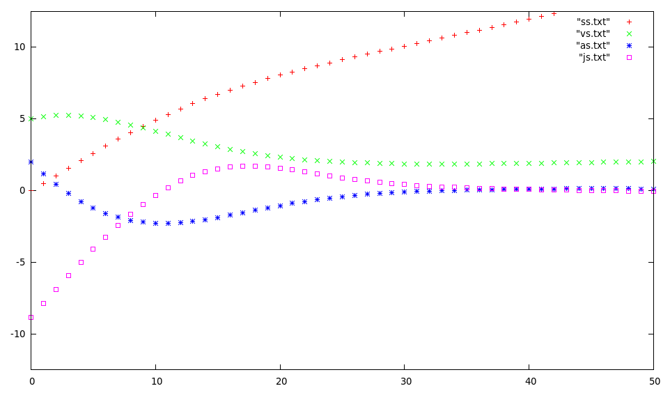
However, this is the first result my optimizer came up with, I optimized the support points for the splines (5 in this example, just conincidence that it's also the chosen time horizon on the horizontal axis).

enter image description here

Compared with the first version with the high degree polynomial, this looks promising!

$\endgroup$
2
  • 1
    $\begingroup$ "inversion of a matrix" - you shouldn't have to invert a matrix; the matrix that often turns up in constructing splines is tridiagonal (or at worst banded), and there are algorithms specially adapted for solving tridiagonal systems that don't need you to have a full $n\times n$ array. $\endgroup$
    – J. M.
    Commented May 20, 2013 at 12:14
  • $\begingroup$ I see, yes, did not deeper look at that. I don't have theoretical knowledge about that, but since my fitness function which constructs the splines may be evaluated several thousand times, I should try to use an off-the-shelf solution here which is maybe optimized. Just a training example for me. $\endgroup$
    – user4344
    Commented May 20, 2013 at 12:17
2
$\begingroup$

If you approximate a function on an interval by polynoms and you have the freedom to choose x, the approximation points, the recommend method is to use gauss quadrature points and the corresponding polynom basis. Once the approximation is obtained you are free to evaluate it of course anywhere in the interval. So use chebyshev polynoms together with chebyshev nodes. This way you won't see any oscillations and you can easily integrate / differentiate the solution on the entire domain.

$\endgroup$

Your Answer

By clicking “Post Your Answer”, you agree to our terms of service and acknowledge you have read our privacy policy.

Not the answer you're looking for? Browse other questions tagged or ask your own question.