How to implement Gauss-Laguerre Quadrature in Python?

Question

To get the hang of Gauss-Laguerre integration I have decided to calculate the following integral numerically, which can be compared to the known analytical solution:

\begin{align} \int_0^{\infty} s^3 \exp(-s^2 t) \, \mathrm{d}t = s \end{align}

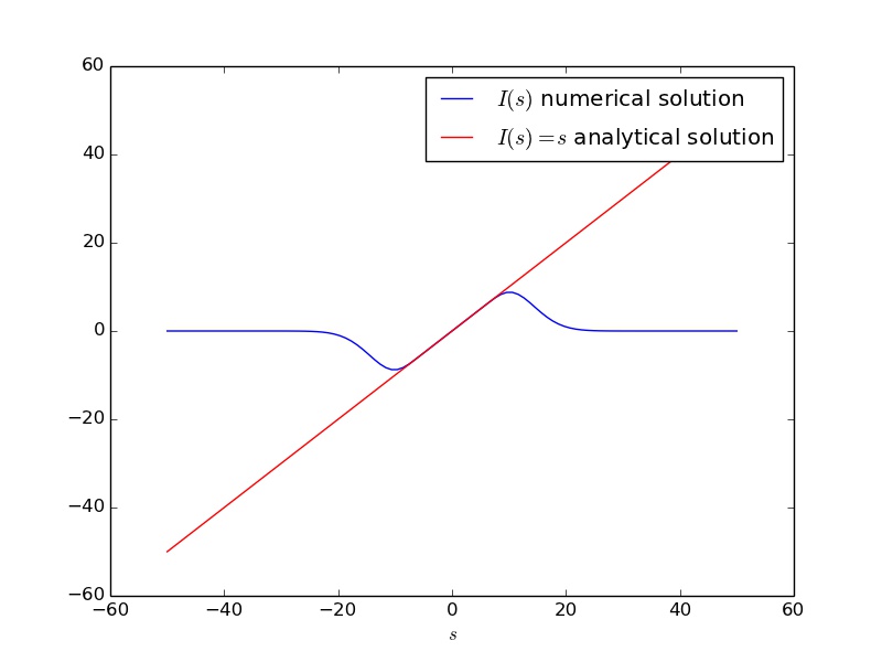
The result can be seen in the graph below. The result matches the analytical solution only on a limited subrange of the independent variable $s$. Evidently more care is needed to ensure convergence of the numerical solution for all $s$. Perhaps the integration routine must be used on smaller subranges? My question is, how can I make Gauss-Laguerre (or Gaussian Quadrature in general) applicable to problems of the kind shown above, where I need the solution to be accurate for all $s$?

import numpy as np
import matplotlib.pyplot as plt


def integrand(t, s):
    return s ** 3 * np.exp(-(s ** 2) * t) * np.exp(t)


vintegrand = np.vectorize(integrand)


def integral(omega):
    I = np.dot(vintegrand(ti, omega), wi)
    return I


vintegral = np.vectorize(integral)


ti, wi, = np.polynomial.laguerre.laggauss(175)


s = np.linspace(-50, 50, 100)

Is = vintegral(s)

plt.plot(s, Is, "b", label="$I(s)$ numerical solution")
plt.plot(s, s, "r", label="$I(s) = s$ analytical solution")
plt.xlabel("$s$")
plt.legend()
plt.show()

Answer 1

The issue here is that the error term increases very quickly as $s$ increases. The error term is, according to this article, is bounded by $$ |E| < \frac{n!^2}{(2n)!}\max |f^{(2n)}(t)|. $$ Now, asymptotically $$ \frac{n!^2}{(2n)!} \approx \frac{\sqrt{\pi n}}{4^n}, $$ and $$ |f^{(2n)}(t)| = s^3(1-s^2)^{2n} e^{-s^2t} < s^3(1-s^2)^{2n}, $$ meaning that the magnitude of the error term bound behaves, approximately, as $$ \propto \left(\frac{1-s^2}{2}\right)^{2n}. $$ This is quite large, and $s$ must be close to $1$ when $n$ is large. This is too pessimistic because these are upper bounds, especially the pessimistic upper bound on $\max|f^{(2n)}|$. In your graph it looks like $s$ can be as large as $10$ or so.

You can avoid this issue by introducing a change of variables $s^2t = u$, that changes the integrand from the form $(\cdots)e^{-s^2t}\,dt$ to the form $(\cdots)e^{-u}\,du$, for which the quadrature rule should be more accurate, because the function multiplying the exponential will not have such fast-growing derivatives. It does make your integral trivial, but it would work on other integrands as well.

Note that this is not an issue with how you invoke the quadrature rule, or that the rule is inapplicable. The issue is that the integrand has very large derivatives, so choosing an equivalent easier integrand should be enough.

Answer 2

You can use QUADPACK through SciPy by modifying your code like this:

# ...

import scipy.integrate

def unweighted(s, t):
    exponent = -s**2*t
    return s**3*np.exp(exponent)

def integral(omega):
    f = functools.partial(unweighted, omega)
    u, v = scipy.integrate.quad(f, 0, np.inf)
    return u

# ...

Answer 3

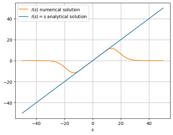
Just for reference, here a simple, fully vectorized implementation with quadpy (a project of mine):

import numpy as np
import matplotlib.pyplot as plt
import quadpy


s = np.linspace(-50, 50, 100)


def integrand(t):
    s2 = s ** 2
    s3 = s2 * s
    return (s3 * np.exp(-np.multiply.outer(s2, t)).T).T * np.exp(t)


scheme = quadpy.e1r.gauss_laguerre(175)
vals = scheme.integrate(integrand)


plt.plot(s, vals, "C1", label="$I(s)$ numerical solution")
plt.plot(s, s, "C0", label="$I(s) = s$ analytical solution")
plt.xlabel("$s$")
plt.legend()
plt.grid()
plt.show()