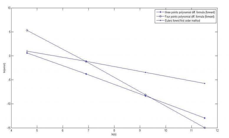
You've chosen a very specific example where the function in question has a single extremely narrow peak and is almost zero everywhere else in the domain. This is an example of a stiff problem where you must take a very tight discretization to resolve the peak. Finite difference approximations are based on polynomial approximations to a curve. In the case where the curve is not locally well-approximated by a polynomial (such as the several grid points that straddle the peak in the Gaussian function here) this can lead to oscillations in the approximating polynomial (see this answer) resulting in a poor estimate of the derivative. Refining the grid eventually leads to a situation where the function is well approximated by a polynomial on the scale of the finite difference stencil and accuracy improves.
As discussed in Jesse Chan's answer, low order methods may actually have lower magnitude errors in some cases. However, I would be skeptical of the accuracy of either method in that case and suggest that you simply need higher resolution.
I tried to replicate your results, but I found that higher order finite differences were actually more accurate (based on RMS error) even in this example. Were you using one sided differences? Here's my matlab script if you want to mess with it.
clear

y = @(x) exp(-32*(x-5).^2);
dydx = @(x) -(64*(x-5)).*y(x);

x=linspace(0,10,50);

%first order (one sided) difference
x1 = x(1:end-1);
dy1 = (y(x(2:end))-y(x(1:end-1)))/diff(x(1:2));

%second order centered difference
x2 = x(2:end-1);
dy2 = (y(x(3:end))-y(x(1:end-2)))/(2*diff(x(1:2)));

%fourth order centered difference
x3 = x(3:end-2);
dy3 = (-y(x(5:end))+8*y(x(4:end-1))-8*y(x(2:end-3))+y(x(1:end-4)))/(12*diff(x(1:2)));

xRef = linspace(0,10,1e5);
dyRef = dydx(xRef);

figure(1)
clf
hold on
plot( xRef, dyRef, 'k' )
plot( x1, dy1,'o')
plot( x2, dy2,'x' )
plot( x3, dy3,'^' )
legend('Analytical','First order','Second order','Fourth order')
title('Computed derivative values')

figure(2)
clf
hold on
plot( x1, abs(dy1-dydx(x1)),'o')
plot( x2, abs(dy2-dydx(x2)),'x' )
plot( x2, abs(dy2-dydx(x2)),'^' )
legend('First order','Second order','Fourth order')
title('Error in the derivative computation')

% rms errors:
sqrt( sum((dy1-dydx(x1)).^2 ) / numel(x1) ) %first order
sqrt( sum((dy2-dydx(x2)).^2 ) / numel(x2) ) %second order
sqrt( sum((dy3-dydx(x3)).^2 ) / numel(x3) ) %fourth order
Please note that this is a slightly different situation than that in the related question. That question was about ODE solvers (Euler and RK). The reason I edited your answer there was to highlight the fact that this case is not typical and that in almost all cases where RK4 is stable it will outperform Euler for a given step size. The ODE analogue to your example here is a stiff ODE where you are not in the stability region of explicit solvers. As I said there, if your ODE solver is unstable all bets are off as far as accuracy (just as all the finite difference methods give poor results on a coarse grid here). Of course a stable low-order implicit method will typically have less error than an unstable explicit method.
Even though you may have "less error" for course grids with the lower order finite differences, the actual errors in your example are huge. In that case, neither solution should be used and you have no choice but to refine the grid or use a different method entirely.
 here y-axis is log(error) and x-axis is log(number of grid points).