1
$\begingroup$

I'm trying to model the Black-Scholes Equation (transformed into a heat equation) using method of lines in Python.

The transformed formula is basically

\begin{equation*} \frac{\partial u}{\partial t} = \frac{\partial^2 u}{\partial x^2} + (k-1)\frac{\partial u}{\partial x} - ku \end{equation*}

where $k$ is a constant and with initial condition

\begin{equation*} u(x,0) = \max(e^x - 1, 0) \end{equation*}

and boundary conditions

\begin{equation*} u(a,t) = \alpha \hspace{35pt} u(b,t) = \beta \end{equation*}

This is python implementation of the method of lines for the above equation should match the results in the matlab code here. I can't seem to find where I went wrong. Any insight on the Python code would be really helpful.

import numpy as np
from scipy.integrate import odeint
import matplotlib.pyplot as plt
from scipy.fftpack import diff as psdiff

N = 40
r = 0.065;
sigma = 0.8;
k = float(0.5*sigma**2);
a = np.log(float(2)/5)
b = np.log(float(7)/5)
t0 = 0;
tf = 5;

x = np.linspace(a, b, N);
xmesh = np.max(np.exp(a)-1,0)*np.ones(x.shape)

def odefunc(u, t):
    dudt = np.zeros(xmesh.shape)

    #boundary conditions
    dudt[0] = u[0]
    dudt[-1] = (7 - 5*np.exp(-k*t))/5 

    #step size
    h = b/(N-1)

    for i in range(1, N-1):
        dudt[i] = ((u[i + 1] - 2*u[i] + u[i - 1]) / h**2) + (k-1)*((u[i] - u[i-1]) / h) - (k*u[i])
    return dudt

tspan = np.linspace(t0, tf, 20);
sol = odeint(odefunc, xmesh, tspan)

for i in range(0, len(tspan), 5):
    plt.plot(xmesh, sol[i], label='t={0:1.2f}'.format(tspan[i]))

# put legend outside the figure
plt.legend(loc='center left', bbox_to_anchor=(1, 0.5))
plt.xlabel('X position')
plt.ylabel('Temperature')

# adjust figure edges so the legend is in the figure
plt.subplots_adjust(top=0.89, right=0.77)
plt.savefig('pde.png')

# Make a 3d figure
from mpl_toolkits.mplot3d import Axes3D
fig = plt.figure()
ax = fig.add_subplot(111, projection='3d')

SX, ST = np.meshgrid(xmesh, tspan)
ax.plot_surface(SX, ST, sol, cmap='jet')
ax.set_xlabel('x')
ax.set_ylabel('t')
ax.set_zlabel('u')
ax.view_init(elev=30, azim=100) # adjust view so it is easy to see
plt.savefig('pde-transient-heat-3d.png')
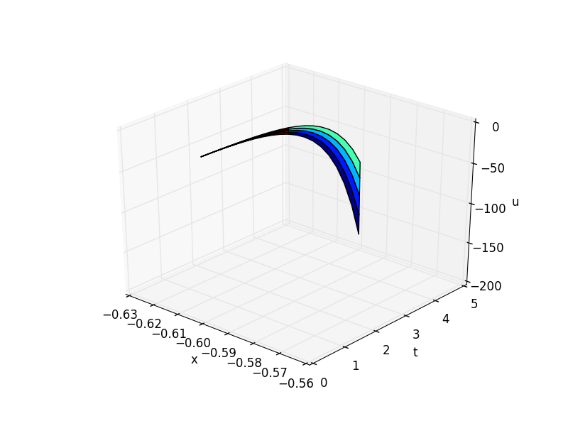
3d Plot

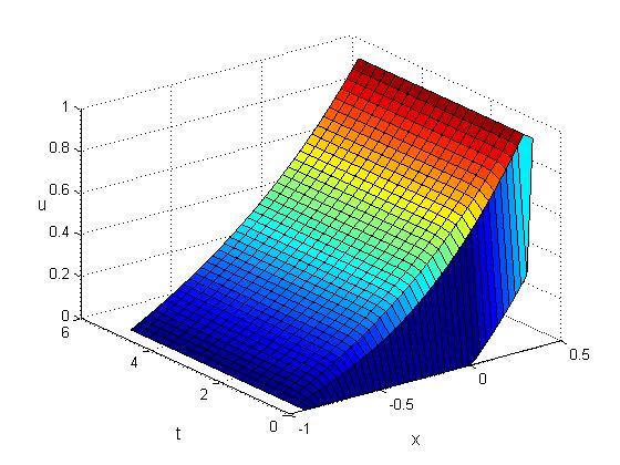
The plot, I believe should look like the following plot

$\endgroup$
4
  • $\begingroup$ Can you state more clearly what is your question? $\endgroup$
    – nicoguaro
    Commented Nov 30, 2015 at 22:06
  • $\begingroup$ I don't think that its all that clear what you are asking. What should the solution look like? I think your plotting is confusing and I am not really sure what the plot should look like on such a narrow range of x. I know Black-Scholes is for option pricing but maybe you could expand on what x and u represent here and choose a better plot (maybe a 2d plot with multiple solutions for each time instead of the 3d plot)? For all I know your plot my be correct and thus there is no question here. $\endgroup$
    – James
    Commented Nov 30, 2015 at 22:06
  • $\begingroup$ oops never mind it looks like nicoguaro has been able to find the solution to your problem after all =). $\endgroup$
    – James
    Commented Nov 30, 2015 at 22:22
  • $\begingroup$ Hi! Thanks for pointing that out. I've edited the question. My python MOL implementation is supposed to match the matlab code for the black-scholes equation. @nicoguaro seems to have pointed out the bug in my code (thanks, by the way!). It still doesn't match the matlab results; I think the problem now is in the variables themselves. $\endgroup$
    – meraxes
    Commented Nov 30, 2015 at 22:43

1 Answer 1

2
$\begingroup$

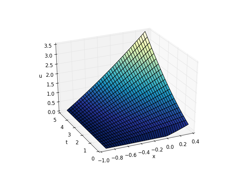
I think that you just plot the wrong thing. The variable xmesh is the initial condition, not the value of x (in your particular case it is constant -0.6). But you don't have the same parameters in your Python and Matlab codes, you are also applying badly your initial conditions.

See here the corrected code (please read it carefully):

from __future__ import division
import numpy as np
from scipy.integrate import odeint
import matplotlib.pyplot as plt
from mpl_toolkits.mplot3d import Axes3D

def odefunc(u, t):
    dudt = np.zeros(x0.shape)

    #boundary conditions
    dudt[0] = u[0]
    dudt[-1] = (7 - 5*np.exp(-k*t))/5 

    #step size
    h = b/(N-1)

    for i in range(1, N-1):
        dudt[i] = (u[i + 1] - 2*u[i] + u[i - 1]) / h**2 +\
                   (k-1)*(u[i] - u[i-1]) / h - k*u[i]
    return dudt


N = 40
r = 0.065;
sigma = 0.8;
k = r/sigma**2
a = np.log(2/5)
b = np.log(7/5)
t0 = 0
tf = 5

x = np.linspace(a, b, N);
x0 = np.exp(x) - 1
x0[x0 < 0] = 0

tspan = np.linspace(t0, tf, 20);
sol = odeint(odefunc, x0, tspan)


#%% Make a 3d figure
fig = plt.figure()
ax = fig.add_subplot(111, projection='3d')

SX, ST = np.meshgrid(x, tspan)
ax.plot_surface(SX, ST, sol, cmap='YlGnBu_r',
                rstride=1, cstride=1)
ax.set_xlabel('x')
ax.set_ylabel('t')
ax.set_zlabel('u')
ax.view_init(elev=30, azim=-115)
plt.savefig('pde-transient-heat-3d.png')
plt.show()

If you plot against x, you obtain this:

enter image description here

$\endgroup$
3
  • $\begingroup$ Thanks for your reply. Trying it in matlab with the pdepe function (see code here) seems to produce a different result however. Any idea on why that would be? $\endgroup$
    – meraxes
    Commented Nov 30, 2015 at 22:30
  • $\begingroup$ Both codes were note equivalent, you need to pay more attention to those details. $\endgroup$
    – nicoguaro
    Commented Nov 30, 2015 at 22:52
  • $\begingroup$ Thanks! In your code, I believe xmesh should be x or x0. But besides that, thanks so much! :) $\endgroup$
    – meraxes
    Commented Nov 30, 2015 at 22:58

Your Answer

By clicking “Post Your Answer”, you agree to our terms of service and acknowledge you have read our privacy policy.

Not the answer you're looking for? Browse other questions tagged or ask your own question.