Statement of the problem
Suppose, we consider the following model $$ \begin{array}{l} (1)~\mathbf{u}_t + \mathbf{F(u)}_x = \mathbf{S}(\mathbf{u},\mathbf{w}), \\ (2)~\mathbf{w}_x = \mathbf{P}(\mathbf{w},\mathbf{u}). \end{array} $$ Computational domain to be as follows $(x,t)=[0,L]\times[0,T]$. Let's consider Neumann boundary conditions (BC) for (1) and initial value problem (IVP) for (2).
Algorithm of simulation as follows: on each time step $t^n$ solve (2) at first and then solve (1).
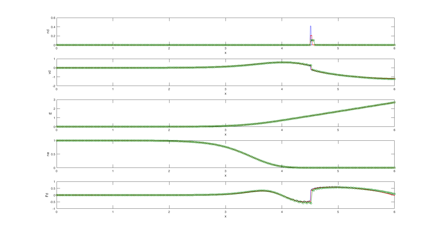
One could assume that $\mathbf{u} = [n_d\,v_d]^T$ and $\mathbf{w} = [n_e\,E]^T$ and obtaion the corresponding plot where $\mathrm{\color{blue}{blue}}$, $\mathrm{\color{red}{red}}$ and $\mathrm{\color{green}{green}}$ lines correspond grids with
$(1024,\,512,\,256)$ poins respectively.
Question
One could realize that the shape of the solution depends on the number of grid points, i.e. grid depence achieved. How to avoid it?
P.S.
Eq. (1) was solved by smoothed Lax-Wendroff scheme (LxW) and eq. (2) was solved by Runge-Kutta scheme of 4th order.