6
$\begingroup$

I'm just doing a very simple experiment. I'm calculating wall shear stress based on Poiseuille flow for a pipe by using lattice Boltzmann method (LBM) and FEM to compare their values with the analytical solution, which is calculated as:

$$\tau = \frac{2 \mu u_\max}{R}$$

Where we have: $u(r) = u_\max \left(1 - (\frac{r}{R})^{2}\right)$ and $\tau = - \mu \frac{\partial u}{\partial r}|_{r=R}$.

For a pipe with $R = 10$mm and $L=100$mm for its radius and length as well as $\mu = 0.004$ $\mathrm{Pa}\cdot\mathrm{s}$ and $u_\max = 0.0125$ $\frac{\mathrm{m}}{\mathrm{s}}$:

$$\tau = \frac{2 \times 0.004 \times 0.0125}{0.01} = 0.01$$

So: $\tau = 0.01$ Pa.

I did the simulation with LBM with a resolution of $0.16$mm and I got the value: $\tau_\text{LBM} = 0.010597292391$ Pa.

On the other hand, I did the simulation with FEM with a resolution of $2$mm and I got: $\tau_\text{FEM} = 0.0097797$ Pa.

You see that the error of FEM is around $2.2$%, but the error of LBM is around $6$%, despite a factor of magnitude coarser resolution of FEM!

For those of you that are familiar with LBM: this LBM simulation is done by using D3Q27 lattice and BFL boundary condition. When I used a simple bounce back instead of BFL, I got $\tau_\text{LBM} = 0.0089005915558$ Pa, which its error is around $11$%.

My main application for using LBM is for a really sensitive biofluidic framework to simulate blood flow in brain arteries. If LBM fails to calculate wall shear stress accurately even in this simple situation of a pipe with Poiseuille flow, how can I trust it to use it for much more complex geometries and flow conditions of blood flow in brain vessels? Why LBM despite its much finer resolution still falls behind the FEM even with a factor of magnitude coarser mesh size? I appreciate any hint or suggestion.

$\endgroup$
3
  • $\begingroup$ Does FEM that you use have hp-refinement enabled? what order of elements is used in FEM? (I am coming from a very different application area, so forgive me if my questions do not apply to the problem you are solving) $\endgroup$
    – Anton Menshov
    Commented Feb 14, 2020 at 23:19
  • $\begingroup$ @AntonMenshov No there is no refinement in FEM framework that I used. Elements are just P1-P1 for velocity and pressure. $\endgroup$ Commented Feb 14, 2020 at 23:26
  • $\begingroup$ This is not related to your immediate question, but P1-P1 elements are not inf-sup stable and you should not use them without pressure stabilization. If possible, use P2-P1 with SUPG stabilization or a DG scheme with P2-P1. $\endgroup$ Commented Aug 16, 2020 at 22:15

2 Answers 2

1
$\begingroup$

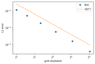
In my opinion issues in LBM like this almost always relate to the boundary condition implementation. Depending on the choice of BC and the way it is implemented it can deteriorate the accuracy of LBM from $O(\delta^2)$ (second-order) to $O(\delta^{1.5})$ or worse to $O(\delta)$ (first-order).

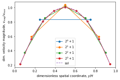
I am not familiar with the specifics of the BFL condition but if I solve this problem with halfway bounceback in a cartesian channel (rather than a pipe) then with as little as three lattice nodes (very rough grid) I get an error in $v_{max}$ of 4%. The numerical solution approaches the analytical solution quite rapidly:
enter image description here enter image description here

With a refinement by doubling the number of nodes yields an error of 1.33%, 0.41%, etc in second-order fashion.

It is not exactly clear to me how you estimate your shear stress but given the equation I assume you determine the max velocity in the pipe and then calculate the stress. So the above errors translate directly to the error in the calculated shear stress. Another option is to determine the stresses directly from the distribution functions.

Now as to why you are getting such relatively large deviations from the FEM solution (which is order of magnitude coarser) I can only provide some potential pointers as I don't have the details of your implementations:

  1. A pipe is axisymmetric system for which generally we want to increase the resolution where the gradients are largest (i.e. at the walls). Standard LBM doesn't account for this as it has a constant lattice spacing but if your FEM solution does account for this you are comparing "apples and oranges".
  2. Furthermore, regarding the axisymmetric system, the equation you provide is a result of solving for poiseuille flow in cylindrical coordinates. Standard LBM is in cartesian coordinates and requires modification for other coordinate systems such as cylindrical coordinates. If your FEM solution is in cylindrical coordinates then again you are comparing "apples and oranges".
  3. Reexamine the boundary condition implementation for any bugs. In my experience this is the largest source of mistakes and one of the points that are most overlooked are the treatment of the corners (where sometimes multiple boundary types come together).
  4. Boundary location (at least for bounce-back) is viscosity dependent, this means that for different values of the relaxation time we can get slight deviations from theory. This is improved by using MRT rather than BGK and in particular by using TRT with a 'magic' relaxation time for which the boundary location is exact to machine precision.

Hope it helps

Code which produced the graphs:

import numpy as np
import matplotlib.pyplot as plt

def sim(n=2, Fo=1):
    """
    """
    ### parameter 
    # D2Q9 lattice
    ns = 9
    cssq = 1/3
    ws = [4/9, 1/9, 1/9, 1/9, 1/9, 1/36, 1/36, 1/36, 1/36]
    ex = [0, +1, 0, -1, 0, +1, -1, -1, +1]
    ey = [0, 0, +1, 0, -1, +1, +1, -1, -1]
    
    # grid
    nx = 1
    ny = 2**n+1
    
    # quantities
    ω = 1
    vmax = 0.01
    ν = cssq*(1/ω-1/2)
    ax = 8*ν*vmax/ny**2
    ay = 0
    
    ### initialization
    rho  = np.ones((nx, ny), dtype=np.float)
    vx = np.zeros((nx, ny), dtype=np.float)
    vy = np.zeros((nx, ny), dtype=np.float)
    
    Fx = np.zeros((nx, ny), dtype=np.float)
    Fy = np.zeros((nx, ny), dtype=np.float)
    
    f = np.zeros((nx+2, ny+2, ns), dtype=np.float)
    ftmp = np.zeros((nx+2, ny+2, ns), dtype=np.float)
    
    # initialize at equilibrium
    for s in range(ns):
        feq = ws[s] # ρ=1, vx=vy=0
        f[1:nx+1, 1:ny+1, s] = feq
        ftmp[1:nx+1, 1:ny+1, s] = feq
    
    ### main loop            
    niter = Fo*int(ny**2/ν)
    for i in range(niter):
    
        ### quantities
        dens = f[1:nx+1,1:ny+1,0]
        momx = 0
        momy = 0
        for s in range(1,ns):
            dens += f[1:nx+1,1:ny+1,s]
            momx += ex[s]*f[1:nx+1,1:ny+1,s]
            momy += ey[s]*f[1:nx+1,1:ny+1,s]
        rho[:,:] = dens 
        
        Fx = dens*ax
        Fy = dens*ay
        
        vx[:,:] = (momx + 0.5*Fx)/dens
        vy[:,:] = (momy + 0.5*Fy)/dens
    
        ### collision
        vv = (vx*vx + vy*vy)/cssq;
        for s in range(ns):
            ev = (ex[s]*vx + ey[s]*vy)/cssq
            feq = ws[s]*rho*(1 + ev + 1/2*ev**2 - 1/2*vv)
            ef = (ex[s]*Fx + ey[s]*Fy)/cssq 
            fforce = (1-1/2*ω)*ws[s]*(
                  (ex[s]-vx + ev*ex[s])*Fx 
                + (ey[s]-vy + ev*ey[s])*Fy
            )/cssq
            ftmp[1:-1,1:-1,s] = (1-ω)*f[1:-1,1:-1,s] + ω*feq + fforce
    
        ### boundaries
        # x boundaries - periodic
        ftmp[0,1:-1,:] = ftmp[-2,1:-1,:]
        ftmp[-1,1:-1,:] = ftmp[1,1:-1,:]
    
        # y boundaries - halfway bounceback
        for (s, so) in zip([2, 5, 6], [4, 7, 8]):
            ftmp[1:nx+1, 0, s] = ftmp[1-ex[so]:nx+1-ex[so], 1, so]
            ftmp[1:nx+1, -1, so] = ftmp[1-ex[s]:nx+1-ex[s], -2, s]
    
        # corners - halfway bounceback
        ftmp[0, 0, 5] = ftmp[0-ex[7], 1, 7]
        ftmp[-1, 0, 6] = ftmp[-1-ex[8], 1, 8]
        ftmp[0, -1, 8] = ftmp[0-ex[6], -2, 6]
        ftmp[-1, -1, 7] = ftmp[-1-ex[5], -2, 5]
    
        ### streaming
        for x in range(1,nx+1):
            for y in range(1,ny+1):
                for s in range(ns):
                    f[x,y,s] = ftmp[x-ex[s], y-ey[s], s]
        
    return dict(
        # vars
        rho = rho,
        vx = vx, vy = vy,
        # params
        nx = nx, ny = ny,
        vmax = vmax,
    )

### figure 1 - numerical vs analytical solutions
errors = []
resolution = []
for n in range(4):
    print(f"running simulation with ny = 2^{n}+1 = {2**n+1}")
    s = sim(n=n)
    vmag = np.sqrt(s['vx']**2 + s['vy']**2)/s['vmax'] # scaled
    yrange, y0, yf = np.arange(s['ny']), -0.5, s['ny']-0.5
    sol = (yrange-y0)*(yf-yrange)/(s['ny']/2)**2
    ϵ = np.linalg.norm(vmag[0,:]-sol)/np.linalg.norm(sol)
    errors.append(ϵ)
    resolution.append(2**n+1)
    plt.plot((np.arange(s['ny'])-y0)/s['ny'], vmag[0,:], '-o', label=f"$2^{n}+1$")

yrange, y0, yf = np.linspace(0,s['ny']-1,100), -0.5, s['ny']-0.5
plt.plot((yrange-y0)/s['ny'], (yrange-y0)*(yf-yrange)/(s['ny']/2)**2, '--', label='sol')

plt.xlabel(r'dimensionless spatial coordinate, $y/H$')
plt.ylabel(r'dim. velocity magnitude, $v_{mag}/v_{max}$')
plt.xlim(0,1)
plt.legend()

### figure 2 - L2 error as function of resolution
plt.loglog(resolution, errors, 'o', basex=2, label='lbm')
plt.loglog(resolution, list(map(lambda r: r**-2, resolution)), '--', basex=2, label=r'$O(\delta^2)$')
plt.xlabel('grid resolution')
plt.ylabel('L2 error')
plt.legend()
$\endgroup$
5
  • $\begingroup$ It doesn’t surprise me that you saw a second-order convergence here cause there is a big hidden assumption here and that is: you assumed all the boundary nodes are halfway from actual cylindrical boundary and by axis symmetry it means your 2D cartesian axisymmetrical framework is identical to a 3D cylindrical coordinate. So it makes sense that you achieved this level of accuracy even with relatively coarse lattice size. If you try to implement a full 3D framework instead of using 2D axisymmetrical model and approximate the cylinder by cartesian voxels, you would see similar worst accuracy. $\endgroup$ Commented Aug 16, 2020 at 23:10
  • $\begingroup$ @AloneProgrammer i don't follow your point; 1. It is not really a hidden assumption as i mention halfway BB, 2. I dont see how the boundary location has to do with the coordinate system rather it is a result of the BC implementation, 3. How can a 2D axisymmetric cartesian framework (which this is actually not as i dont use symmetry) be identical to a 3D cylindrical coordinate framework? It would be missing terms related to the curvature of the pipe $\endgroup$
    – nluigi
    Commented Aug 17, 2020 at 6:56
  • $\begingroup$ @AloneProgrammer should i assume that in your simple bounce back implementation you dont have the boundaries halfway between nodes? In that case you would have Full bounce back which is known to be first-order accurate and may explain the deviations for that implementation. $\endgroup$
    – nluigi
    Commented Aug 17, 2020 at 7:01
  • $\begingroup$ If you read the question carefully, you would find that I used BFL for boundary condition primarily, although I reported the halfway bounce back result as well. My point is that: Your model is 2D. When you use a 2D model to solve a 3D model like this in a pipe, you assume that everything is axisymmetric. But, in my implementation, my code only takes 3D models and it doesn't care about any symmetry in the geometry and generally use a graph-based unstructured model to voxelize any 3D geometry into cartesian voxels... $\endgroup$ Commented Aug 17, 2020 at 15:53
  • $\begingroup$ It means lattice sites at 0$^{\circ}$, 90$^{\circ}$, 180$^{\circ}$ and 270$^{\circ}$ are halfways from the actual cylindrical boundary. In other directions, there might be a deviation from halfway. Overall, it means if you revolve your 2D axisymmetric geometry you would get a pipe that is different from my 3D voxelized model and that's the reason why you actually working on a cylindrical coordinate but my model works on a cartesian coordinate. In another word, you exploit symmetry of cylinder but my LBM framework because is written generally for unstructured models doesn't care about symmetry. $\endgroup$ Commented Aug 17, 2020 at 15:55
0
$\begingroup$

Try D3Q17 for axisymmetric problem. To my knowledge D3Q27 is developed for Cartesian coordinate system. Unless the radial coordinate system properly simulated, then it is difficult to get correct answer with less error.

$\endgroup$
1
  • $\begingroup$ I don't have D3Q17 in my LBM implementation and I never heard of it honestly. But, even if I had it, it won't help me, cause at the end my geometries are not axisymmetric at all and if I understand correctly D3Q17 is designed specifically for axiysmmetric geometries and just gives good result for pipe, which has axisymmetry, still I can't use it for complex shapes without axisymmetry. $\endgroup$ Commented Feb 18, 2020 at 20:35

Your Answer

By clicking “Post Your Answer”, you agree to our terms of service and acknowledge you have read our privacy policy.

Not the answer you're looking for? Browse other questions tagged or ask your own question.