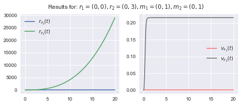
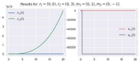
Goal:
I want to use Python to illustrate how a magnetic dipole with magnetic moment m2 moves in a non-homogeneous magnetic field in a 2D-Plane. This field is generated by another magnetic dipole with moment m1. However, I get results that are not plausible.
For the calculation of the trajectory of m2 I use the equations from wiki - force between magnets
Theoretical Background:
Given is a magnetic dipole with constant moment m1 and constant position r1!. m1 generates a magnetic flux density
$${\displaystyle \mathbf {B}_1 (\mathbf {r} )={\frac {\mu _{0}}{4\pi }}{\frac {3\mathbf {\hat {r}} (\mathbf {\hat {r}} \cdot \mathbf {m} )-\mathbf {m} }{|\mathbf {r} |^{3}}}\qquad (1)}$$
where r is a vector from the center of the magnetic dipole to the location where the magnetic field is measured. In this non-homogeneous magnetic field a magnetic dipole with moment m2 and position r2 is placed. Its magnetic field can be neglected B2 = 0.
Only the dynamics of m2 shall be considered. According to the linked Wikipedia page, m2 will be subjected to a torque D and a force F. The torque is neglected D=0. The magnetic moment m2 is therefore constant.
Due to the acting force, the position vector r_2(t) depends on time. Its time evolution is obtained from the solution of the equation of motions, which is my objective:
$$ \frac{d^2}{dt^2}\mathbf{r}_2 (t) = \binom{\dot{r}_{2x}}{\dot{r}_{2y}} = \mathbf{F}$$
According to Wikipedia, m1 exerts the following force on m2: (r = r2 - r1, r = ||r||_2):
$$\begin{align} \mathbf{F} &= \nabla |\mathbf{m}_2\cdot \mathbf{B}_1| \qquad(3) \\\\ &= {\frac {1}{ r^{5}}}\left[(\mathbf {m} _{1}\cdot \mathbf {r} )\mathbf {m} _{2}+(\mathbf {m} _{2}\cdot \mathbf {r} )\mathbf {m} _{1}+(\mathbf {m} _{1}\cdot \mathbf {m} _{2})\mathbf {r} -{\frac {5(\mathbf {m} _{1}\cdot \mathbf {r} )(\mathbf {m} _{2}\cdot \mathbf {r} )}{r^{2}}}\mathbf {r} \right] \qquad (4) \\ &= \frac{\mathbf{m}_1 \mathbf{r}}{r^5} \mathbf{m}_2 + \frac{\mathbf{m}_2\mathbf{r}}{r^5}+\frac{\mathbf{m}_1\mathbf{m}_2}{r^5}\mathbf{r} - \frac{5(\mathbf{m}_1 \mathbf{r})(\mathbf{m}_1\mathbf{r})}{r^7}\mathbf{r}\\\\ &= \mathbf{c}_1 + \mathbf{c}_2 + c_3 (\mathbf{r}_2 - \mathbf{r}_1) - c_4 (\mathbf{r}_2 - \mathbf{r}_1) \qquad (5)\\\\ &= \mathbf{c}_1 + \mathbf{c}_2 + \mathbf{r}_1 (c_4 - c_3) + \mathbf{r}_2 (c_3 - c_4)\qquad (6)\\\\ &= \mathbf{c}_1 + \mathbf{c}_2 + \mathbf{c} + d\cdot\mathbf{r}_2, \quad \mathbf{c}_1, \mathbf{c}_2, \mathbf{c}\in \mathbb{R}^2, d\in\mathbb{R} \qquad (7) \end{align} $$
The introduced variables c1,c2, c, d should be self-explanatory. Now we can define 4 ODEs and solve them numerically with the Runge-Kutta method:
$$\begin{align} \dot{r}_{2x} &= v_{2x} \qquad (8)\\\\ \dot{r}_{2y} &= v_{2y} \qquad (9)\\\\ \dot{v}_{2x} &= c_{1x} + c_{2x} + c_x + d\cdot r_{2x} \qquad (10)\\\\ \dot{v}_{2y} &= c_{1y} + c_{2y} + c_y + d\cdot r_{2y} \qquad (11)\\\\ \end{align}$$
What to expect?
An attractive force should act on the magnet m2, so that
$$ t \gg 1: \mathbf{r}_2 = \mathbf{r}_1 $$
My Results
m2 is repelled instead of being attracted.
Probably I made a mistake in the implementation. But I have already checked it several times and found no error... Does anyone of you know what went wrong
Python 3 Code
import numpy as np
import matplotlib.pyplot as plt

"""
Important quantites that will influence the dynamics

m1:  Magnetic Moment of the dipole that creates a constant magnetic field
m2:  Magnetic Moment of a dust particle
r1:  Position of m1: r1(t) = const
r2:  Position of m2: r2(t) will depend on time
"""

# Constants
m1 = np.array([0, 1], float)
m2 = np.array([0, -1], float)
r1 = np.array([0, 0], float)

# Initial conditions of the of m2 R = [r2_x, r2_y, v2_x, v2_y]
R = np.array([0, 3, 0, 0], float)


def distance(r1, r2, n):
    """
    computes the distance ||.||_2 between position r1 and r2
    """

    return np.linalg.norm(r1 - r2) ** (n)

def pre_factors(r1, r2, m1, m2):
    """
    Computes the prefactors in the equation of motion
    d^2 r2 / dt^2 = F = c1 + c2 + c + r2 * d   r2,c1,c2,c € R^2, d € R
    """

    r = r2 - r1
    l = distance(r1, r2, 5)

    c1 = ( np.dot(m1, r) * m2 ) / l
    c2 = ( np.dot(m2, r) * m1 ) / l

    c3 = np.dot(m1, m2) / l
    c4 = ( 5 * np.dot(m1, r) * np.dot(m2, r) ) / distance(r1, r2, 7)

    c = (c4 - c3) * r2
    d = c3 - c4

    return c1, c2, c, d

def f(r1, R, m1, m2):
    """
    now we can compute the righthand side of the four 1st order ODEs:
    d/dt r2_x = v2_x
    d/dt r2_y = v2_y
    d/dt v2_x = c1_x + c2_x + c_x + d*r2_x
    d/dt v2_y = c1_y + c2_y + c_y + d*r2_y
    """

    r2x = R[0]
    r2y = R[1]
    v2x = R[2]
    v2y = R[3]

    c1, c2, c, d = pre_factors(r1, R[:2], m1, m2)

    f_r2x = v2x
    f_r2y = v2y
    f_v2x = c1[0] + c2[0] + c[0] + d * r2x
    f_v2y = c1[1] + c2[1] + c[1] + d * r2y

    return np.array([f_r2x, f_r2y, f_v2x, f_v2y], float)


# Constants for the Simulation
a = 0.0  # t_0
b = 20.0  # t_end
N = 1000 # number of iterations
h = (b-a) / N # time step, e.g. h = (100 - 0) / 1000 = 0.1s

# Create lists to store the computed values
tpoints = np.arange(a,b+h,h)

xpoints, ypoints = [], []
vxpoints, vypoints = [], []

for dt in tpoints:
    #print(R)
    xpoints.append(R[0])
    ypoints.append(R[1])
    vxpoints.append(R[2])
    vypoints.append(R[3])

    # Runge-Kutta-4th Order Method
    k1 = dt * f(r1, R, m1, m2)
    k2 = dt * f(r1, R + 0.5 * k1, m1, m2)
    k3 = dt * f(r1, R + 0.5 * k2, m1, m2)
    k4 = dt * f(r1, R + k3, m1, m2)
    R += (k1 + 2*k2 * 2*k3 + k4)

plt.style.use('seaborn')
fig, axes = plt.subplots(nrows=1, ncols=2, figsize=(8, 3))
axes[0].plot(tpoints, xpoints, label = '$r_{x_2}(t)$')
axes[0].plot(tpoints, ypoints, label = '$r_{y_2}(t)$')

axes[0].legend()

axes[1].plot(tpoints, vxpoints,'r', label = '$v_{x_2}(t)$', alpha = 0.5)
axes[1].plot(tpoints, vypoints, 'k',label = '$v_{y_2}(t)$', alpha = 0.5)
axes[1].legend()

fig.suptitle("Results for: $r_1 = (0,0), r_2 = (0,3),  m_1 = (0,1), m_2 = (0,-1)$")
#plt.savefig("2.pdf" , format='pdf',  bbox_inches="tight")
fig.tight_layout()

