preconditioner for Laplace "without" boundary values

Question

I'm looking at solving systems with the FEM discretization $$ -\int_\Omega (\Delta u) v = \int_\Omega \nabla u \cdot \nabla v - \int_\Gamma (n\cdot\nabla u) v. $$ without applying Dirichlet- or Neumann-type boundary conditions. The resulting matrix is generally not self-adjoint (except in for 1D meshes).

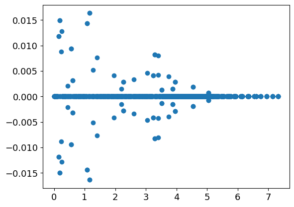
The kernel consists of all linear functions over the domain, so there are always $n+1$ eigenvalues 0 (where $n$ is the dimensionality of the mesh).

The right-hand side is such that the system is consistent and I would like to find a solution of the system. The idea is to use GMRES, starting off with an all-zero initial guess.

Is there a good preconditioner for this known in literature? I played around with Dirichlet- and Neumann-Laplace without much success.

---

To get a feel, here's how to create the matrix and plot the spectrum in sckit-fem:

import matplotlib.pyplot as plt
import meshzoo
import numpy as np
import skfem
from skfem.helpers import dot, grad


@skfem.BilinearForm
def laplace(u, v, _):
    return dot(grad(u), grad(v))


@skfem.BilinearForm
def flux(u, v, w):
    return dot(w.n, u.grad) * v


points, cells = meshzoo.disk(6, 20)

pT = np.ascontiguousarray(points.T)
cT = np.ascontiguousarray(cells.T)
mesh = skfem.MeshTri(pT, cT)

element = skfem.ElementTriP1()

basis = skfem.CellBasis(mesh, element)
facet_basis = skfem.FacetBasis(basis.mesh, basis.elem)

lap = skfem.asm(laplace, basis)
boundary_terms = skfem.asm(flux, facet_basis)

A = lap - boundary_terms

out = np.linalg.eigvals(A.toarray())
plt.plot(out.real, out.imag, "o")
plt.savefig("out.png", bbox_inches="tight")
plt.show()

Answer 1

Here is at least an idea, whether it works is a different question.

Let's say you sort unknowns so that you have the ones in the interior of the domain first, and then all those at the boundary. Then the matrix that corresponds to your problem decomposes in the following way: $$ A = \begin{pmatrix} A^{\circ\circ} & B^{\circ\partial} \\ C^{\partial\circ} & D^{\partial\partial} \end{pmatrix} $$ where $\circ$ indicates shape functions in the interior and $\partial$ on the boundary of the domain. $A^{\circ\circ}$ is simply the Dirichlet-boundary condition matrix for the Laplace operator and we know how to invert it efficiently. One could then think about using a Schur complement approach where you first solve for the boundary unknowns and then the interior unknowns, or maybe the other way around.

If you follow the arguments of the Silvester-Wathen preconditioner for the Stokes system, you will also be able to construct a good preconditioner for the whole matrix based on the Schur complement approach; it will probably look something like this: $$ P^{-1} = \begin{pmatrix} A^{\circ\circ} & B^{\circ\partial} \\ 0 & S^{\partial\partial} \end{pmatrix}^{-1} $$ where $S^{\partial\partial}=D^{\partial\partial}-D^{\partial\circ}[A^{\circ\circ}]^{-1}B^{\circ\partial}$ is the Schur complement. It would be worthwhile thinking about whether one can approximate $S^{\partial\partial}$ by a simpler matrix, in the same way as for the Stokes equations, one approximates the Schur complement by the mass matrix.

Answer 2

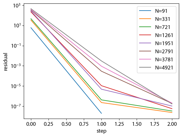
As others have pointed out, (algebraic) multigrid can actually be a good preconditioner in this scenario. Below is a proof-of-concept implementation with scikit-fem and pyamg. It shows that pyamg's preconditioner makes the number of GMRES iterations more or less independent of the number of unknowns.

I only tested this with a mesh of a few thousand unknowns. The main computational cost is computing the left nullspace of A, used for making the right-hand side consistent. (A computation that isn't necessary in the actual application where consistency is guaranteed.)

import matplotlib.pyplot as plt
import meshzoo
import numpy as np
import pyamg
import scipy.linalg
import scipyx
import skfem as fem
from skfem.helpers import dot
from skfem.models.poisson import laplace

rng = np.random.default_rng(0)

tol = 1.0e-8

for n in range(5, 41, 5):
    # points, cells = meshzoo.rectangle_tri((0.0, 0.0), (1.0, 1.0), n)
    points, cells = meshzoo.disk(6, n)
    print(f"{n = }, {len(points) = }")

    @fem.BilinearForm
    def flux(u, v, w):
        return dot(w.n, u.grad) * v

    mesh = fem.MeshTri(points.T.copy(), cells.T.copy())
    basis = fem.InteriorBasis(mesh, fem.ElementTriP1())
    facet_basis = fem.FacetBasis(basis.mesh, basis.elem)

    lap = fem.asm(laplace, basis)
    boundary_terms = fem.asm(flux, facet_basis)

    A = lap - boundary_terms

    b = rng.random(A.shape[1])
    # make the system consistent by removing A's left nullspace components from the
    # right-hand side
    lns = scipy.linalg.null_space(A.T.toarray()).T
    for n in lns:
        b -= np.dot(b, n) / np.dot(n, n) * n

    ml = pyamg.smoothed_aggregation_solver(
        A,
        coarse_solver="jacobi",
        symmetry="nonsymmetric",
        max_coarse=100,
    )
    M = ml.aspreconditioner(cycle="V")

    _, info = scipyx.gmres(A, b, tol=tol, M=M, maxiter=20)
    # res = b - A @ info.xk

    num_unknowns = A.shape[1]
    plt.semilogy(
        np.arange(len(info.resnorms)), info.resnorms, label=f"N={num_unknowns}"
    )

plt.xlabel("step")
plt.ylabel("residual")
plt.legend()
plt.savefig("out.png", bbox_inches="tight")
plt.show()

Answer 3

If you are not enforcing any boundary conditions, you should remove the nullspace of the problem (to make sure that there is a unique solution, MatSetNullSpace can be used to achieve this in PETSc) and then use multigrid on the problem (for example, PCMG of PETSc).

What surprises me is that there are n+1 zero eigenvalues. I would expect only one. Are you solving the Laplace's equation on surfaces (like a 2D surface embedded in 3D space) and the boundary is the boundary of that surface (like 1D boundary embedded in 3D space)? That is the only scenario I can imagine that the nullspace is that populous.