I'm trying to implement the Rusanov flux as a global matrix for solving a PDE. The Rusanov flux for an element (e) and its neighbouring element (k) reads: $$f^{(*, e, k)}=\frac{1}{2}\left[f^{(e)}+f^{(k)}-\hat{\mathbf{n}}^{(e, k)}\left|\lambda_{\max }\right|\left(q^{(k)}-q^{(e)}\right)\right].$$ The first term is just the average of both flux values at the element boundary and the second term includes the jump operator (The second term is a dissipation term that modifies the flux and helps with discontinuities in the solution). The second term is the term that gives me a headache, because in my solution it just doesn't do anything and my solver works better without it, so it is probably implemented wrong.
The Problem: Im trying to solve a simple advection problem $$\partial _t u +\partial_x f(u) =0.$$ Writing this in the weak form introduces a boundary term where a numerical flux needs to be introduced (since the field has two values at each element interface). I implemented the numerical flux as two global matrices $A$ and $B$. This way I was able to write the numerical flux in the form $$A*f(u) + B*u$$ with $$f(u)=(f(u(x_1)), f(u(x_2)),f(\hat u(x_2)),f(u(x_3)),...,f(u(x_n))$$ and $$u(x)=f(u)=(u(x_1), u(x_2),\hat u(x_2), u(x_3),...,u(x_n).$$ This is for just two interpolation points within an element. I introduced the hat notation to show that the field can have two distinct values at the same x value. For the polynomial expansion of my solution I used Lagrange Polynomials with the nodal property $$L_i(x_j)= \delta _{ij}$$. Since the boundary term includes the Lagrange Polynomial $$[L_i(x) f^*(u)]^{x_{right}} _{x_{left}}$$ and due to their nodal property only one boundary term can survive, depending on the Lagrange Polynomial. From this I obtained the following local form for the matrices $$A= \begin{bmatrix} 1/2 & 1/2 \\ -1/2 & -1/2 \end{bmatrix} $$ and $$B= \lambda _{max}\begin{bmatrix} 1/2 & -1/2 \\ 1/2 & -1/2 \end{bmatrix} $$ A minus sign has been included in the second row because the boundary term is evaluated on the left element interface here. In global form the would have the form $$A= \begin{bmatrix} 0 & & & \dots & &0 \\ 0& 1/2 & 1/2 & 0 & \dots & 0 \\ 0 & -1/2 & -1/2 & 0 & \dots & 0 \\ \vdots & & & \ddots \\ \end{bmatrix} $$ I've implemented this and the dissipation term seems to have a bug. When excluding it equation are solved nicely. But when moving to more complex PDE's this dissipation term is needed to keep the solution stable.
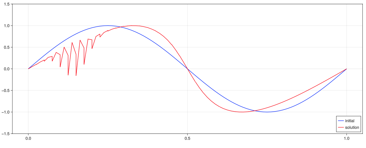
Note: Another bug I have notices is that, with the dissipation term included I'm only able to solve equation where the wave moves from the right to the left. The other way the solution quickly becomes unstable (I. have included the figure illustrating this).
I have also included a code sample where the global $A$ and $B$ matrices are constructed.
Ne: Number of Elements N: Polynomial order for expansion
function lax_friedrich_1(N :: Int64, Ne :: Int64,)
    L_e = [1/2 1/2; -1/2 -1/2]
    L_G = zeros(N*Ne, N*Ne)
    for n in 1:Ne-1
        L_G[N*n:N*n+1, N*n:N*n+1] = L_e
    end
    #Periodic boundary conditions
    #L_G[1,1]=-1/2
    #L_G[1,Ne*N]=-1/2
    #L_G[N*Ne,N*Ne]=1/2
    #L_G[N*Ne,1]=1/2
    #---
    L_G[1,1]=-1.0
    L_G[N*Ne,N*Ne]=1.0
    return L_G
end
function lax_friedrich_2(N :: Int64, Ne :: Int64, u::Vector{Float64}, flux_derivative::Function)
    L_e = [1/2 -1/2; 1/2 -1/2]
    L_G = zeros(N*Ne, N*Ne)
    for n in 1:Ne-1
        c=max(abs(flux_derivative(u[N*n])), abs(flux_derivative(u[N*n+1])))
        L_G[N*n:N*n+1, N*n:N*n+1] = c*L_e
    end
    #Periodic boundary conditions
    #L_G[1,1]=1/2*max(abs(flux_derivative(u[1])), abs(flux_derivative(u[end])))
    #L_G[1,Ne*N]=-1/2*max(abs(flux_derivative(u[1])), abs(flux_derivative(u[end])))
    #L_G[N*Ne,N*Ne]=-1/2*max(abs(flux_derivative(u[end])), abs(flux_derivative(u[1])))
    #L_G[N*Ne,1]=1/2*max(abs(flux_derivative(u[1])), abs(flux_derivative(u[end])))
    #---
    #Symmetric boundary conditions L[1,1], L[N*Ne,N*Ne] are already set to 0
    return L_G
end