Context
I want to solve a 1D Burgers equation with a discontinuous Galerkin approach on the space-time domain $(x,t)\in [0,1]^2$. I want to project the function $u(x) = e^{-\frac{(x-0.5)^2}{0.02}}$ over basis functions. The choosen basis are normalized Legendre polynomials.
The DG representation of the initial state is then: $$u^{DG}(x) = \sum_k <\phi_k, u> \phi_k(x)$$ with test function $\phi_k$, the dot product $<f,g> = \int_{\Omega} f(x)g(x)dx$ and $\Omega = [0,1]$ the full space domain.
Problem
To answer the above problem, integrals need to be computed. For every test function $v$ (defined over the physical domain $[a,b]\in [0,1]$ not the reference one) and its associated test function over the reference element $\hat{v}$, I want to compute: $$ \begin{align} \int_a^b u(x) v(x)dx &= \frac{b-a}{2}\int_{-1}^1 u(f^{-1}(y)) \hat{v}(y)dy = \frac{b-a}{2}\sum_k w_k u(f^{-1}(y_k)) \hat{v}(y_k) \end{align} $$ The first equality is obtained with the variable substitution $y = f(x) = \frac{2(x-a)}{b-a}-1$. The second one is obtained by using a Gauss-Legendre quadrature scheme on $[-1,1]$ with weights $w_k$ and abscissas $x_k$. By using the above formulae, I do not get a good projection of the initial state over the Galerkin basis. But when I remove the $\frac{b-a}{2}$ factor the results look right. I do not get what I did wrong in the integration. The results can be seen by running the code below. Do not hesitate to ask for clarifications.
Prolematic snippet
# dot product over reference element /!\ jacobian missing
    U[ie*p + i] += np.sum(weightQuadrature*u0(xPhysical)*basisFunctionOnQuadraturePointArray[i])

    # supposed to work
    #U[ie*p + i] += J*np.sum(weightQuadrature*u0(xPhysical)*basisFunctionOnQuadraturePointArray[i])
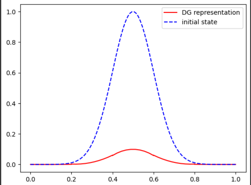
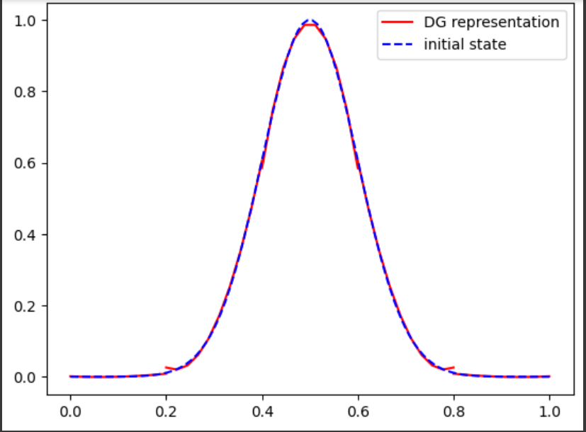
Results with 5 elements and a quadratic polynomial basis
With the "correct" quadrature scheme:
By removing the Jacobian of the transformation from the physical domain to the reference element (removing the factor):
Full Code
import numpy as np
import matplotlib.pyplot as plt

############
# reference element + quadrature
############
x1ref, x2ref = -1.0, 1.0
QuadratureRule = np.array([
    [0.3607615730481386,    0.6612093864662645],
    [0.3607615730481386,    -0.6612093864662645],
    [0.4679139345726910,    -0.2386191860831969],
    [0.4679139345726910,    0.2386191860831969],
    [0.1713244923791704,    -0.9324695142031521],
    [0.1713244923791704,    0.9324695142031521],
])
xQuadrature = QuadratureRule[:,1]
weightQuadrature = QuadratureRule[:,0]
nQuadrature = len(QuadratureRule)

del(QuadratureRule)

def integrateOnReferenceElement(func):
  return integrateOnReferenceElement_(func, weightQuadrature, xQuadrature)

def integrateOnReferenceElement_(func, weightQuadrature, xQuadrature):
  return np.sum(weightQuadrature*func(xQuadrature))
############
# basis functions definition (Legendre)
############
p = locdim = 3
basisFunctionArray = [
         np.polynomial.legendre.Legendre([0]*i+[1]) for i in range(p)
]

# normalizing the basis functions
for i in range(p):
  new_coeff = 0.0

  basisFunctionI = basisFunctionArray[i]

  def basisFunctionI_2(x):
    return basisFunctionI(x)**2

  norm_2 = integrateOnReferenceElement(basisFunctionI_2)
  new_coeff = 1/np.sqrt(norm_2)
  basisFunctionArray[i].coef[-1] = new_coeff

  norm_2 = integrateOnReferenceElement(basisFunctionI_2)
  assert np.isclose(norm_2,1)

# saving values of basis functions on quadrature points
basisFunctionOnQuadraturePointArray = []

for i in range(p):
    basisFunctionOnQuadraturePointArray.append(basisFunctionArray[i](xQuadrature))

basisFunctionOnQuadraturePointArray = np.stack(basisFunctionOnQuadraturePointArray, axis=0)

############
# space mesh
############
nElt = 10
nPts = nElt + 1
X = np.linspace(0, 1, nPts)
elementConnectivityArray = np.array([[i, i+1] for i in range(nPts-1)])

############
# project initial state on basis
############
def u0(x):
  return np.exp(-(x-0.5)**2/0.02)

nDof = p * nElt

# vector representation of u0 in the discontinuous Galerkin basis
U = np.zeros(nDof)

for ie in range(nElt):
  tag1, tag2 = elementConnectivityArray[ie]
  x1, x2 = X[tag1], X[tag2]
  l = np.abs(x2-x1)

  # jacobian of the transformation from the real domain to reference element
  J = l/2

  # quadrature points on the real/physical space
  xPhysical = l * (xQuadrature + 1)/2 + x1

  for i in range(p):
    # dot product over reference element /!\ jacobian missing
    U[ie*p + i] += np.sum(weightQuadrature*u0(xPhysical)*basisFunctionOnQuadraturePointArray[i])

    # supposed to work
    #U[ie*p + i] += J*np.sum(weightQuadrature*u0(xPhysical)*basisFunctionOnQuadraturePointArray[i])

############
# plotting result function
############
x_test = np.linspace(-1,1, 10)

for ie in range(nElt):
  tag1, tag2 = elementConnectivityArray[ie]
  x1, x2 = X[tag1], X[tag2]
  l = np.abs(x2-x1)
  J = l/2
  xReal = l * (x_test + 1)/2 + x1
  yReal = 0.0

  # representation over the local element
  for i in range(p):
    yReal = yReal + U[ie*p + i] * basisFunctionArray[i](x_test)
  plt.plot(xReal, yReal, c='r')

x_ = np.linspace(0,1, 1000)

plt.plot(x_, u0(x_), label='initial state', c='b', linestyle='--')
plt.legend()

