2
$\begingroup$

This is an attempt to reproduce Moon et al. 1995, and the author's copy can be obtained through here.

As a benchmark, we estimate the time-lagged mutual information of a simple sine signal $\sin(0.02\pi t)$ using Gaussian kernels: $$K(y)=\dfrac{\exp\left(-\dfrac{(y-y_i)^TS^{-1}(y-y_i)}{2h^2}\right)}{(2\pi)^{d/2}h^d\det(S)^{1/2}},$$ where $h$ is chosen to be $$h=\left\{\dfrac{4}{(d+2)}\right\}^{1/d+4}n^{-1/(d+4)},$$ where $d$ is the dimension of the multivariate kernel, and $n$ is the number of data points.

I wrote a Matlab function (the code is at the end of the post).

Suppose $x_t$ is the original time series $\sin(0.02\pi t)$ with 400 data points $t=1,2,\cdots,400$, and $x_{t-\tau}$ is $\sin[0.02\pi (t-\tau)]$. The author plotted the estimated mutual information $I_{x_t,x_{t-\tau}}$ as a function of $\tau$:
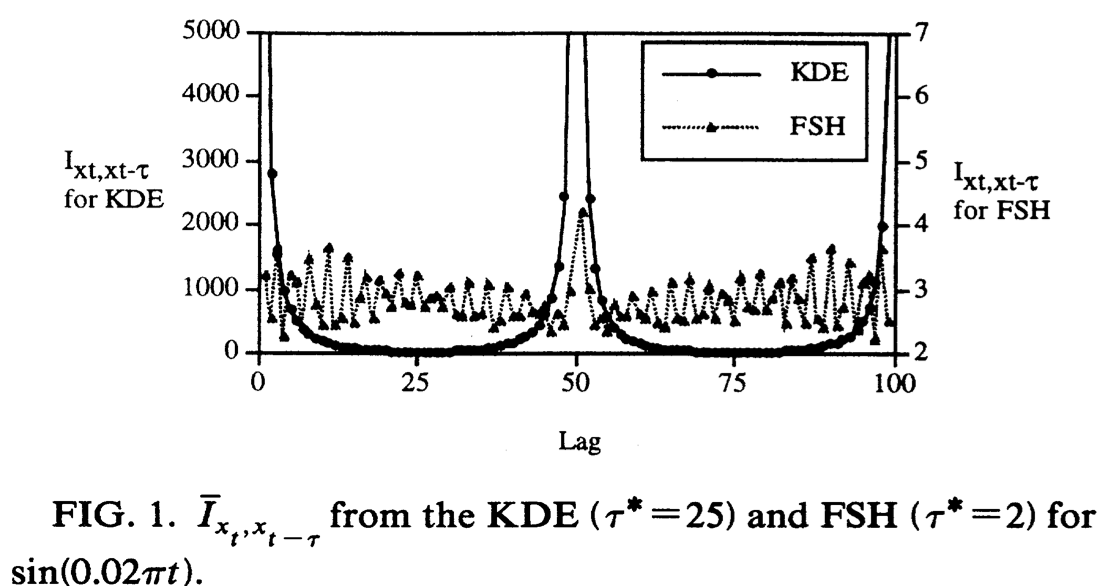
enter image description here

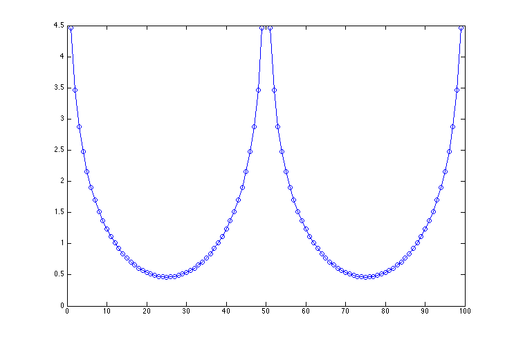
However, what I got from my code is

enter image description here

While the qualitative features (like the diverging mutual information at lag 0, 50 and 100), but the magnitude is far off and the overall shape is not right.

My 1st suspicion is the fact that I used different window widths for joint pdf and marginal pdf, and they may not be consistent. So my question is: how to consistently construct joint and marginal pdf estimate in the context of mutual information estimation?

Second question is: is there anything wrong in the code besides the possibly inconsistent pdf KDEs?

Edit 1:

The reason why I choose KDE over other methods is that I think KDE is simple and intuitive in concept and possibly also simple in implementation. Besides MI, I also want to estimate transfer entropy and possibly other information-theoretic measures as well. I feel that estimating joint probability is general enough to apply on various information-theoretic measures. Please let me know if you have comment on my argument above.

I didn't use anything that can be found only in Matlab. Code in R, Python, etc. is welcome.

Edit 2: the Matlab code

The Matlab code:

function [MI] = get_MI(xt, xt_lag)
% xt is original time series, xt_lag is the lagged one, both are column
% vectors
x_pair = [xt' xt_lag']; n=length(xt);

d=1; h_d1=(4/(d+2))^(1/(d+4)) * n^(-1/(d+4));

d=2; h_d2=(4/(d+2))^(1/(d+4)) * n^(-1/(d+4));

MI = 0.;

Sxy_pair = cov(x_pair); invS_pair = Sxy_pair\eye(2); detS_pair = det(Sxy_pair);

Sxy_xt = cov(xt'); invS_xt = Sxy_xt\eye(1); detS_xt = det(Sxy_xt);

Sxy_lag = cov(xt_lag'); invS_lag = Sxy_lag\eye(1); detS_lag = det(Sxy_lag);

for ix=1:n
    Psq = p_mkde(x_pair(ix,:)', x_pair', h_d2, invS_pair, detS_pair);
    Ps = p_mkde(x_pair(ix,1), xt, h_d1, invS_xt, detS_xt);
    Pq = p_mkde(x_pair(ix,2), xt_lag, h_d1, invS_lag, detS_lag);

    MI = MI + (log2(Psq) - log2(Ps) - log2(Pq));
end

MI = MI/n;

end

function [pxy]=p_mkde(x,X,h,invS,detS)

s1=size(X);
d=s1(1);
N=s1(2);

pxy_sum=0;
for ix=1:N
    p2=(x-X(:,ix))'*invS*(x-X(:,ix));
    pxy_sum=pxy_sum+1/sqrt((2*pi)^d*detS)*exp(-p2/(2*h^2));
end
pxy=1/(N*h^d)*pxy_sum;
end
$\endgroup$
6
  • $\begingroup$ It may be the case that the original picture was simplified because it's three in one. In particular, the sine has to be below 1, but it's not. $\endgroup$
    – James
    Commented Oct 1, 2014 at 18:59
  • $\begingroup$ A general comment: it's much easier to estimate MI than to estimate the joint density. If MI is all you need, you might want to consider directly estimating MI (or entropies. E.g. by using a nearest neighbor based estimator). $\endgroup$
    – Memming
    Commented Oct 1, 2014 at 22:25
  • $\begingroup$ @James, what did you mean by "simplified"? I don't understand your argument. $\endgroup$
    – wdg
    Commented Oct 2, 2014 at 2:11
  • $\begingroup$ @Memming, actually my purpose is to learn about KDE technique. Besides MI, I also need transfer entropy and possibly other information-theoretic measures so that I need an estimate method that is general enough like KDE. $\endgroup$
    – wdg
    Commented Oct 2, 2014 at 2:13
  • $\begingroup$ @wdg if you can estimate MI, KL-div and entropy, most of the other information-theoretic quantities including transfer entropy can be easily estimated. I recommend you NOT to estimate the joint density unless you have a low (<5) dimensional problem and A LOT of data. $\endgroup$
    – Memming
    Commented Oct 3, 2014 at 15:20

1 Answer 1

3
+25
$\begingroup$

Let me start by restating that this is a terrible MI estimation procedure. Please don't use this in any serious business, unless you are absolutely sure you know what you are doing.

You are making two critical mistakes in your code:

  1. Your scale doesn't match because you didn't do the integration properly. Mutual information is defined as in the paper is for probability, not probability density. But your kernel density estimator gives you back probability density which integrates to one, but does not sum to one on the points on a grid. If you want to use the sum formula as in the paper, you need to convert the density back to probability.

  2. You are adding the probabilities only at the points where your data live, and counting multiple times on those regions. You should be integrating over the support of the entire distribution! An easy way to do this would be to make a uniform grid to integrate over. I think you should carefully review the definition of mutual information. (You need to add the probabilities, not the point wise MI estimates over the data.)

This is not a code-review site, but a couple of small things on your code.

  • never use reserved matlab function names as variables: sum is one of them
  • You don't need inv, so don't use it. Use \ and / instead
  • try not to use i as a looping variable. i is for imaginary numbers in MATLAB (so is j)
  • hint: MATLAB has a KDE for 1D which you can verify your code against: ksdensity

EDIT: I misinterpreted the code. I was wrong. OP is replacing expectation with sum over samples, so there's no problem using density nor having a grid.

$\endgroup$
3
  • $\begingroup$ Thanks for the comments on the code. Regarding your point 1.: I understand your point. How can I convert the density back to probability in the context of kernel density estimate? $\endgroup$
    – wdg
    Commented Oct 5, 2014 at 11:15
  • $\begingroup$ In response to your point 2., I add only the probabilities of the data point, because I'm using resubstitution estimate: $H_n=-\frac{1}{n}\sum_{i=1}^n\log f_n(X_i)$. If the underlying process of the time series is ergodic, then time average is as good as ensemble average. $\endgroup$
    – wdg
    Commented Oct 5, 2014 at 12:23
  • $\begingroup$ @wdg Aha. Sorry for not understanding your code. If you are replacing expectation by sum over samples, then it's hard to correct for point 1. But, the units in the denominator should cancel the units in the numerator, so I actually think I was totally wrong now. :'( $\endgroup$
    – Memming
    Commented Oct 6, 2014 at 13:34

Your Answer

By clicking “Post Your Answer”, you agree to our terms of service and acknowledge you have read our privacy policy.

Not the answer you're looking for? Browse other questions tagged or ask your own question.