2
$\begingroup$

I'm trying to design the frequency response function for a low-pass filter. I need the function to be polynomial and to fulfill the following constraints: the coefficients must sum to 1, the function must lie at the interval [0, 1] and its' value at 1 must be 1.

Inspired by this StackExchange answer, I've tried to solve this problem using an SDP solver. The only non-trivial constraints for the program are the bounds for the polynomial. I implemented them by requiring the polynomial to correspond to a quadratic form defined by a positive semidefinite matrix. Using the same method, I can require the polynomial to be monotonic by imposing a nonnegativity constraint on the polynomial's derivative.

Here is an example of a solution to the above: enter image description here
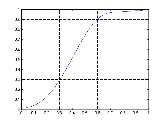
Here, the polynomial is required to be monotonic and to pass at two control points which are at the intersections of the dashed-lines on the chart. The latter is supposed to model the transition region of the filter.

The problem is that the filter in the chart is very far from the ideal low-pass filter. This is because the SDP solver fails when I try to shrink the transition region. Another thing that happens when I do that is that the quadratic form's matrix condition number skyrockets. I suspect that these two things are related. Raising the polynomial's order doesn't help.

Any suggestions about how to solve this issue?

$\endgroup$
2
  • $\begingroup$ What's preventing you from solving $\min \|y-Vp\|^2$ s.t. $p\ge 0$? $\endgroup$ Commented Mar 14, 2012 at 14:58
  • $\begingroup$ I assume that by p you mean the coefficients of the polynomial. When I restrict them to be nonnegative, the approximation error at the control points is huge. $\endgroup$ Commented Mar 14, 2012 at 15:56

1 Answer 1

3
$\begingroup$

By forcing your control points close to each other, your Vandermonde matrix becomes nearly singular and hence the condition number is poor and your solver fails.

For simplicity, you have $x_2=x_1+\epsilon$, where $x_i$ are your control points. The two corresponding Vandermonde rows are:

$$ \begin{align}\left(\begin{matrix} 1 & x_1 & x_1^2 &\cdots & x_1^n\\ 1 & x_2 & x_2^2 &\cdots & x_2^n \end{matrix}\right) &= \left(\begin{matrix} 1 & x_1 & x_1^2 &\cdots & x_1^n\\ 1 & x_1+\epsilon & x_1^2(1 + O(\epsilon)) &\cdots & x_1^n(1+O(\epsilon)) \end{matrix}\right) \\ & \approx \left(\begin{matrix} 1 & x_1 & x_1^2 &\cdots & x_1^n\\ 1 & x_1 & x_1^2 &\cdots & x_1^n \end{matrix}\right) \end{align} $$

The ideal low-pass filter response is discontinuous. A polynomial approximation will invariably exhibit the Gibbs phenomenon. Constraining the polynomial to monotonicity potentiates the problem.

$\endgroup$
3
  • $\begingroup$ Setting the x-coordinates of the control points to 0.4 and 0.6, the condition number of the Vandermonde matrix is below 8. The condition of the matrix Q (defined in the link I gave), however, is above 10^6. $\endgroup$ Commented Mar 13, 2012 at 22:21
  • $\begingroup$ That is correct, but the matter remains unchanged. I've updated the answer. $\endgroup$ Commented Mar 14, 2012 at 12:25
  • 1
    $\begingroup$ Maybe Runge's phenomenon is more applicable here. $\endgroup$ Commented Mar 14, 2012 at 15:26

Your Answer

By clicking “Post Your Answer”, you agree to our terms of service and acknowledge you have read our privacy policy.

Not the answer you're looking for? Browse other questions tagged or ask your own question.