Order of Accuracy Measurements on 1D Advection Methods

Question

I am trying to learn about basics of computational fluid dynamics, at the moment on the simple example of linear advection in 1D. I am am currently testing the theoretical predictions of the order of accuracy of different methods, and the results that I am finding are not what I would expect them to be, and I don't understand why.

First point would be testing how the order of accuracy behaves with decreasing cell width dx. For piecewise constant upwind differencing advection in 1D, i.e. advecting a quantity $q$ with constant positive velocity $u$, the equation is

$$ q^{n+1}_i = q^n_i + \frac{u \Delta t}{\Delta x} \left( q_{i-1} - q_i \right) $$

This method is, on paper, of order $\mathcal{O}(\Delta x)$. (e.g. section 3.6 of these lecture notes).

However, going from a piecewise constant to a piecewise linear reconstruction should give us a second order accurate method in space. On a smooth initial condition, this should hold even when slope limiters are employed, which reduce the order of accuracy in regions of non-monotone states to first order.

So I tested the accuracy on a smooth Gaussian profile in a periodic "box" of size 1:

dx = 1./nx
for i in range(nx):
    x = (i+0.5)*dx
    rho[i] = 1 + 2 * np.exp(-((x-0.5)**2/0.05))

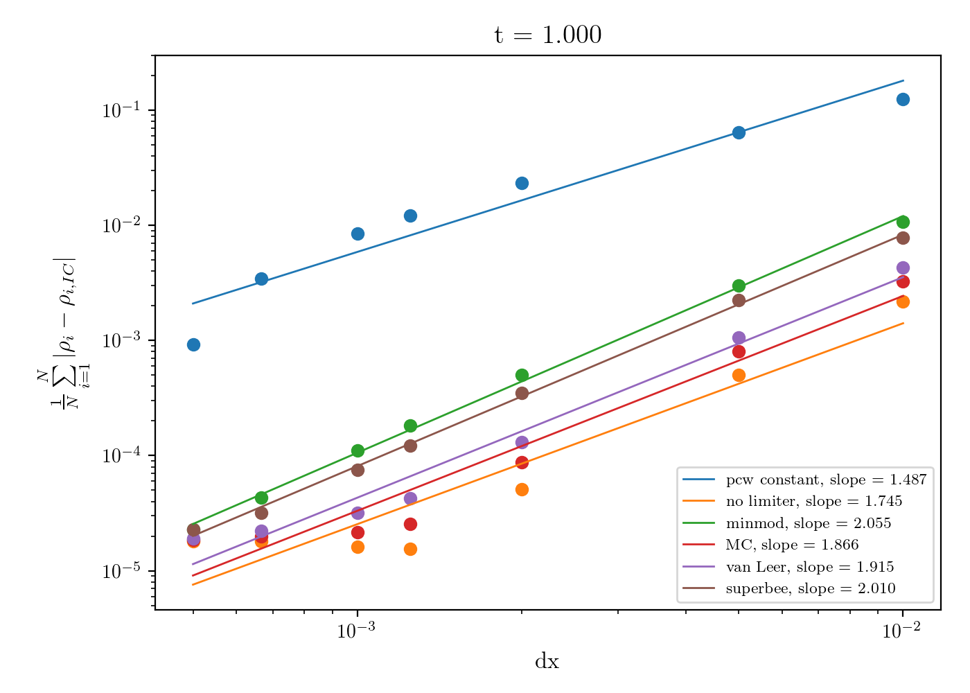
and then run the simulation up to $t = 1$ with $u = 1$, such that the analytical solution should be exactly the initial conditions again. To remove any time dependence, I enforced a small constant time step for all choices of dx, such that every choice of dx needs to do exactly the same number of steps to get to $t = 1$. Then I plotted the $L1$ norm of the results compared to the initial conditions vs dx, and fitted a line to compute the slope of the plot.

This is the result:

About this plot, I have two things that I don't understand fully:

Question 1: for piecewise constant advection, I expect a slope of $1$, but get $\approx 1.5$. Why is that? My understanding is that the order of accuracy estimation gives you the minimal order of accuracy, but in certain cases, it can be higher. Is that correct?

Question 2: for piecewise linear advection, specifically when using no slope limiter, the monotonized centered limiter (MC), and the van Leer limiter, the curve isn't linear any more, but plateaus for small dx. Why is that?

---

Secondly, I wanted to measure the order of accuracy of the time variable. I expect all the methods mentioned earlier to be $\mathcal{O}(\Delta t)$.

Also, following this answer, I expect the introduced error $$ Err = \frac{c\Delta x}{2}\frac{\partial^2 u}{\partial x^2}(1-C_{cfl}) \propto -C_{cfl} $$

i.e. to be $\mathcal{O}(C_{cfl})$, where $C_{cfl} \leq 1$ is the user-set Courant number.

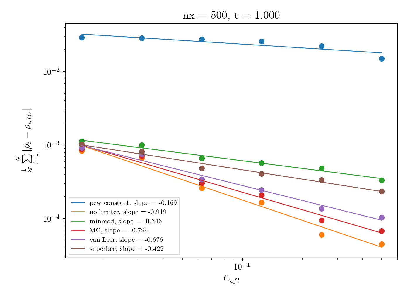
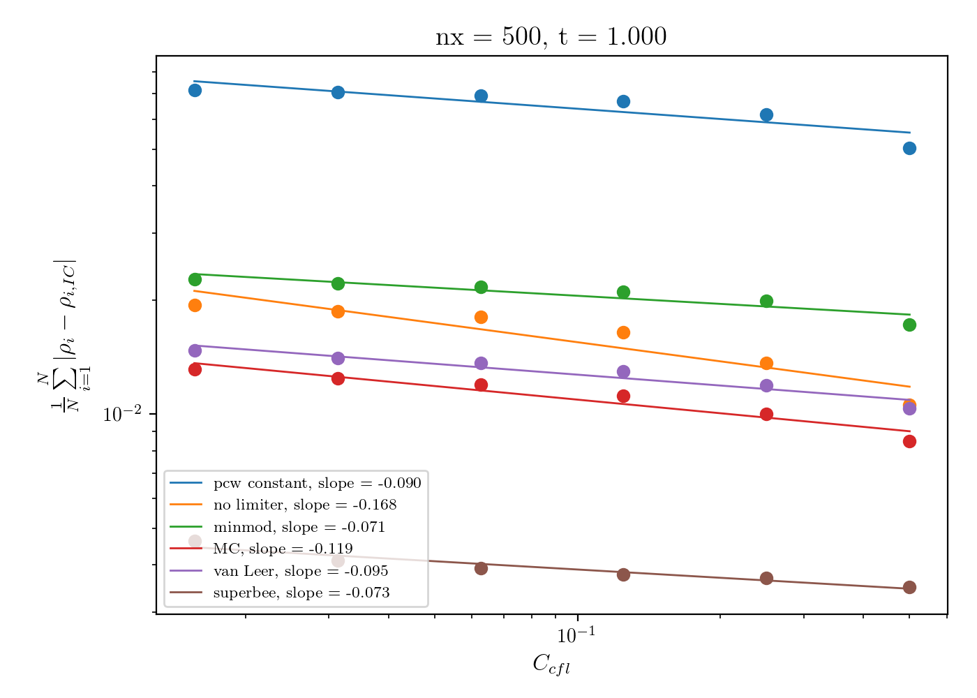
So I ran the same initial conditions for a fixed dx up to $t = 1$ again with different Courant numbers, expecting to get a slope $\approx 1$. However, the resulting curves show a line often closer to slope $0$:

In fact, it gets even worse if instead of a Gaussian profile I use a step function as initial conditions:

dx = 1./nx
for i in range(nx):
    center = (i+0.5)*dx
    if center > 1./3 and center < 2./3:
        rho[i] = 2
    else:
        rho[i] = 1

Then all lines are closer to slope $0$ than $1$:

This leads to another two questions for me:

Question 3: Why aren't the slopes close to $1$?

Question 4: Why does the initial condition change the accuracy of the $C_{cfl}$ dependence so drastically? Compare for example the piecewise linear advection without a slope limiter between the Gaussian profile and the step functoin. The slope drops from $\approx 0.9$ to $\approx 0.15$.

---

Edit: corrected equation

Answer 1

Ok, so I think I figured it out.

Question 1: for piecewise constant advection, I expect a slope of $1$, but get $\approx 1.5$. Why is that? My understanding is that the order of accuracy estimation gives you the minimal order of accuracy, but in certain cases, it can be higher. Is that correct?

Yes. The order of convergence gives you an upper limit for the introduced error. In practice, and depending on the case you're solving, the error can be smaller and the method can converge faster than the order of magnitude of the upper error limit predicted by theory.

Question 2: for piecewise linear advection, specifically when using no slope limiter, the monotonized centered limiter (MC), and the van Leer limiter, the curve isn't linear any more, but plateaus for small dx. Why is that?

I am actually not sure exactly why. It could be accumulation of errors, or the flattening of the smooth functions through the limiters. However, it is not important as such, because forcing the same time step on all simulations actively reduces $C_{cfl}$ for smaller $nx$, i.e. higher $dx$.

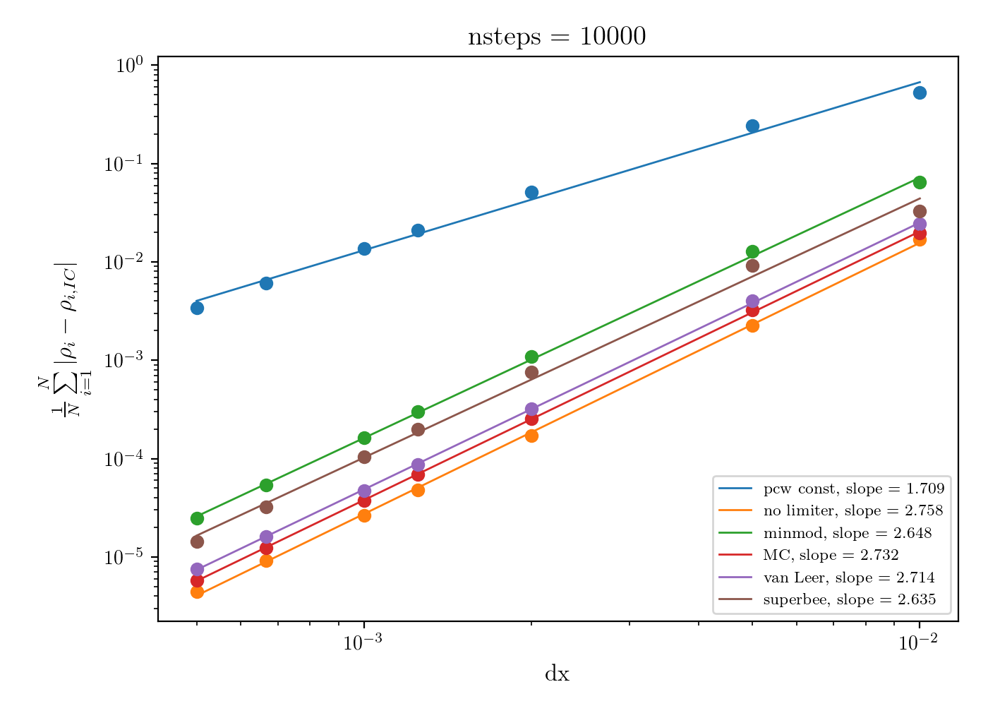
So in order to have a fair comparison on space dependence, you need to let the simulation run for **exactly the same number of steps with a fixed initial condition, and the same $C_{cfl}$. As stated by the equation $$Err = \frac{c\Delta x}{2}\frac{\partial^2 u}{\partial x^2}(1-C_{cfl}) \propto -C_{cfl} ~~~~~~(1)$$ modifying $C_{cfl}$ also modifies the diffusivity of the method. So we need to keep all those quantities fixed, and run the simulation the exact same number of steps in every case for a good comparison. (I was just too lazy to implement the computation of the analytical solution at non-integer times in the evaluation scripts...)

Following that recipe, this is the result (again for the Gaussian profile):

We get almost perfect power laws.

Question 3: Why aren't the slopes close to $1$?

Because I was measuring the wrong thing again.

Firstly, to measure the dependence on the time step choice, again we need to perform the exact same number of time steps and then compare to the analytical solution.

Secondly, equation (1) is a quantification of the diffusivity of the method, not an expression of the upper error boundary depending on time. However, we need to take it into account when we want to show the dependence on $\Delta t$.

In the following, focus only on the piecewise constant advection (blue dots and lines), as I don't have the theory present for the piecewise linear scheme to back up my findings. What makes things more difficult is that for the piecewise linear advection, $\Delta t$ also enters the computation of the fluxes between the cells, thus also affects the spatial component. It is not trivial to separate between the $\Delta x$ and $\Delta t$ dependence in these cases.

So let us focus on the piecewise constant method.

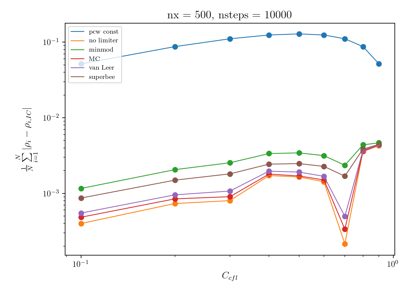
Here is what we get for enforcing $10000$ time steps for $0.1 \leq C_{cfl} \leq 0.9$:

The blue line is clearly not following any power law. The reason is that with decreasing $C_{cfl}$, the diffusive term in eqn. (1) increases.

Therefore, in order to measure the $\Delta t$ dependence of the method, we need to go to values of $\Delta t$ where moving from one $\Delta t_1$ to a smaller $\Delta t_2$ has barely any effect on the diffusive term.

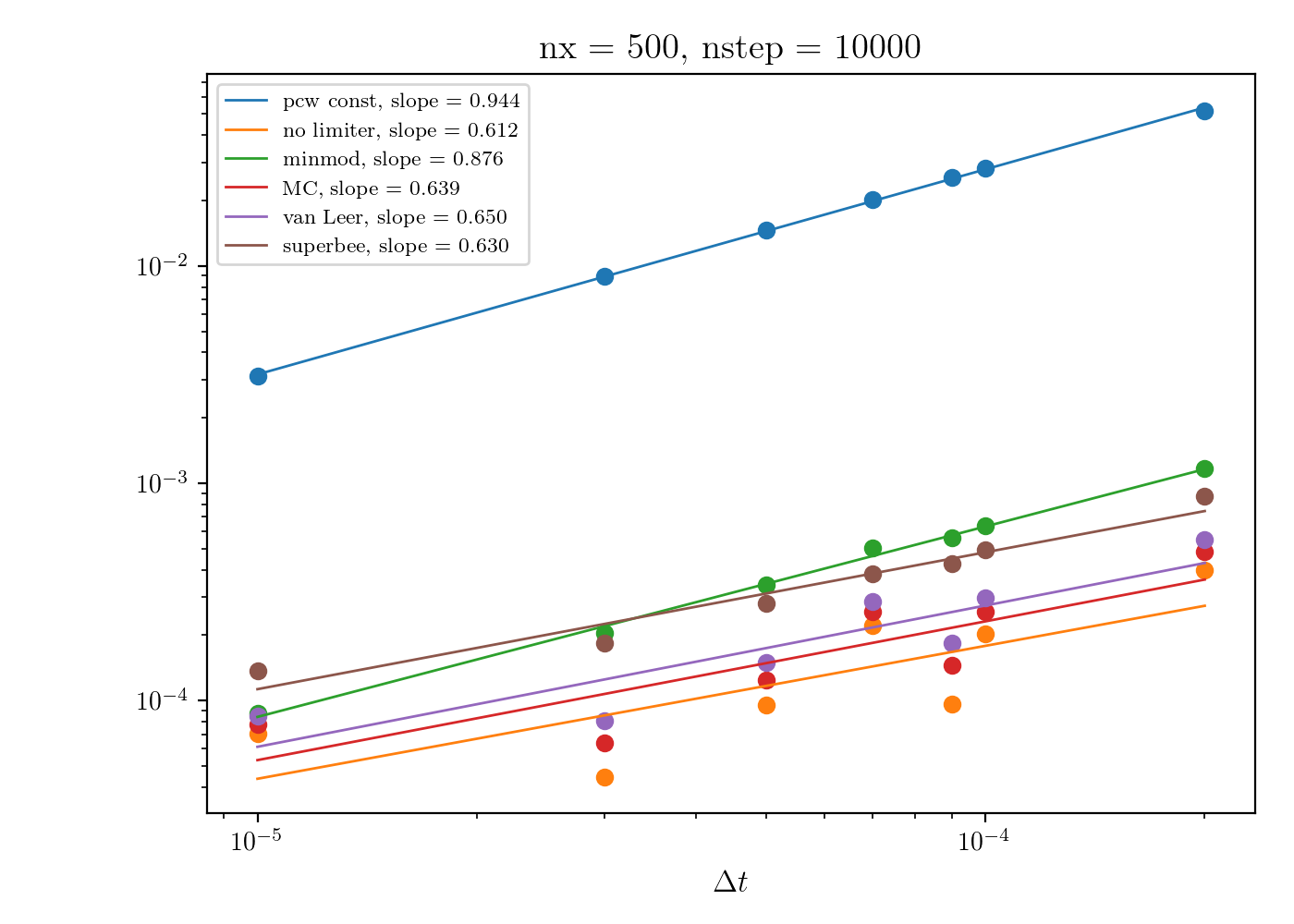
And indeed, when the highest $\Delta t$ corresponds to $C_{cfl} = 0.001$, the result is:

And we obtain almost a perfect power law with the slope $\approx 1$. (Again, focus only on the blue line.)

Question 4: Why does the initial condition change the accuracy of the $C_{cfl}$ dependence so drastically? Compare for example the piecewise linear advection without a slope limiter between the Gaussian profile and the step functoin. The slope drops from $\approx 0.9$ to $\approx 0.15$.

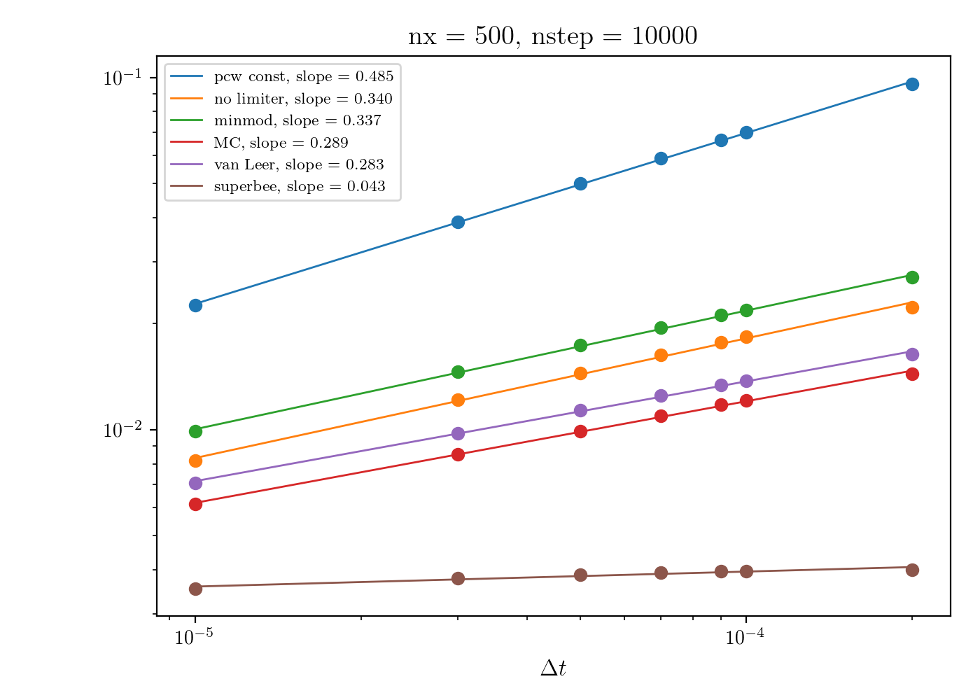
Because the derivation of the order of convergence estimate assumes a smooth initial condition, such that you can take derivatives and do Taylor expansions, which is not given for discontinuities. Following R. LeVeque's "Finite Volume Methods for Hyperbolic Problems", chap. 8.6, it can be shown that for the first order piecewise constant advection, the error goes as $$ Err \propto \sqrt{ \Delta x ~ t } $$

So if we have constant time steps $\Delta t$, $t = N \Delta t$, and keeping $N$ constant we should have:

$$ Err \propto \sqrt{ \Delta x ~ \Delta t } $$

for discontinuous initial conditions.

And indeed, using the step function described in the question, we get the following $\Delta t$ dependence:

with a nice slope of $\approx 0.5$