Solving the eigenvalue from a set of coupled second order differential equation numerically

Question

I met a problem in solving a set of coupled differential equation, as shown below:

$$A_1\psi_1(z)+A_2\frac{d^2\psi_1(z)}{dz^2}+A_3\frac{d\psi_2(z)}{dz}=\lambda\psi_1(z)$$ $$A_4\psi_2(z)+A_5\frac{d^2\psi_2(z)}{dz^2}+A_3\frac{d\psi_1(z)}{dz}=\lambda\psi_2(z)$$ with the following 4 boundary condition:

$$\psi_1(0)=\psi_1(d)=0$$ $$\psi_2(0)=\psi_2(d)=0$$

where $A_{i}$ is a constant coefficient.

I've been stuck in this question for a long time. As the coupling term $A_{3}$ present in the problem. Without the boundary condition on the first order derivative, I was unable to determine the value of $\lambda$. Is there any numerical method to solve this type of eigenvalue problem?

Answer 1

This problem can be interpreted as a coupled convection-diffusion-reaction equation in two variables. You can use the Finite Element Method to solve it. Must be mentioned that you need to use some form of stabilisation for the convection term. You can use SUPG (Streamline Upwind Petrov Galerkin) stabilisation.

After discretisation, we can write it in the form the generalised eigenvalue problem

\begin{equation} \mathbf{K} \mathbf{\Psi} = \lambda \mathbf{M} \mathbf{\Psi}, \end{equation} which can be solved for $\lambda$(s).

You can refer to this textbook for the details.

I would be happy to discuss further if you want.

Answer 2

You can rewrite the problem in matrix form as

$$\begin{bmatrix} A_1 + A_2 \frac{d^2}{dz^2} &A_3\frac{d}{dz}\\ A_3\frac{d}{dz} &A_4 + A_5\frac{d^2}{dz^2} \end{bmatrix}\begin{Bmatrix} \psi_1\\ \psi_2\end{Bmatrix} = \lambda \begin{Bmatrix} \psi_1\\ \psi_2\end{Bmatrix}\, ,$$

that can be thought as

$$\mathcal{L} \Psi = \lambda \Psi\, ,$$

where $\mathcal{L}$ is your matrix operator and $\Psi$ is your vector variable.

Thus, you can think of methods for solving it. The following pop to my mind:

• Finite differences.

• Weighted residuals:

  • Galerkin (such as FEM).
  • Collocation.

Since you have a problem in 1D, I would try with finite differences or collocation first.

Answer 3

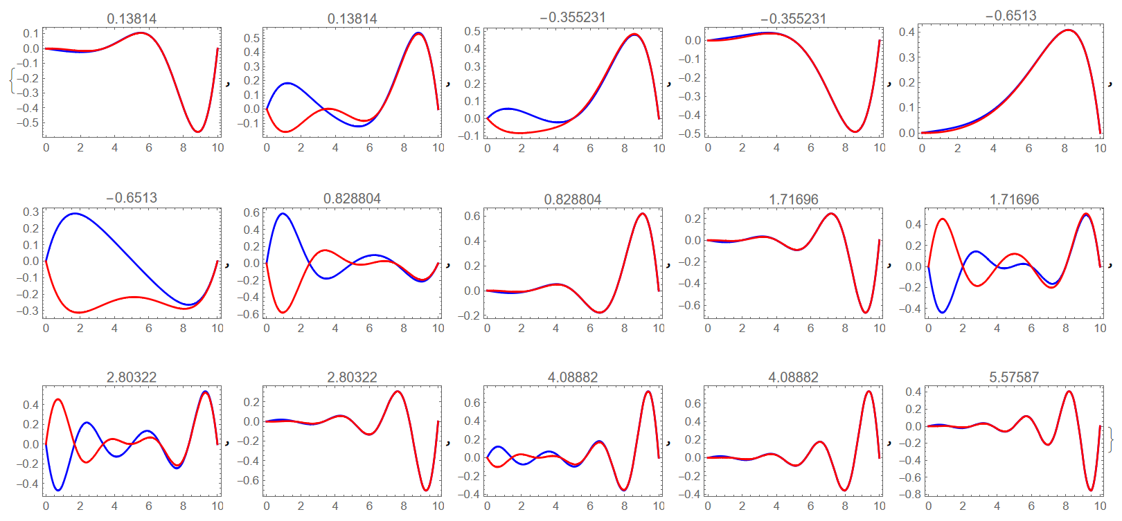
We can show how the eigensystem looks like for a given $A_i, d$, for example, in a case of $A_1=A_4=-1, A_2=A_5=-1,A_3=1$ and $d=10$ we have (in the pictures below $\psi_1$ - blue,$\psi_2$ - red, $\lambda$ is shown under pictures)

Answer 4

The differential equations can also be written as the following system of first order differential equations

$$ \frac{d}{dz}x(z) = M\,x(z), \tag{1} $$

with $x(z)=\begin{bmatrix}\psi_1(z) & d/dz\,\psi_1(z) & \psi_2(z) & d/dz\,\psi_2(z)\end{bmatrix}^\top$ and

$$ M = \begin{bmatrix} 0 & 1 & 0 & 0 \\ \frac{\lambda-A_1}{A_2} & 0 & 0 & -\frac{A_3}{A_2} \\ 0 & 0 & 0 & 1 \\ 0 & -\frac{A_3}{A_5} & \frac{\lambda-A_4}{A_5} & 0 \\ \end{bmatrix}. $$

The solution to these differential equations can be obtained using

$$ x(z) = e^{M\,z} x(0), \tag{2} $$

using the matrix exponential, defined as

$$ e^X = \sum_{n=0}^\infty \frac{1}{n!}X^n = I + X + \frac{1}{2} X^2 + \cdots. $$

The first constraints can also be written as that $x(0)$ has to lie in the following span

$$ \left\{\begin{pmatrix}0\\1\\0\\0\end{pmatrix},\begin{pmatrix}0\\0\\0\\1\end{pmatrix}\right\}. $$

The last constraints requires that $x(d)$ lies in that same span, which is equivalent that it lies orthogonal to the its null space. This is equivalent to

$$ \begin{bmatrix} 1 & 0 & 0 & 0 \\ 0 & 0 & 1 & 0 \end{bmatrix} e^{M\,d} \begin{bmatrix} 0 & 0 \\ 1 & 0 \\ 0 & 0 \\ 0 & 1 \end{bmatrix} = \begin{bmatrix} 0 & 0 \\ 0 & 0 \end{bmatrix}. \tag{3} $$

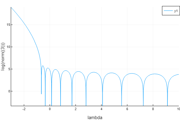
By taking some norm, such as the Frobenius norm, of the left hand side of $(3)$ the eigenvalue problem becomes a root finding problem. Though, I am not sure if this would be the easiest way of solving this, but I thought it might be worth mentioning (but would be too long for a comment).

---

For example when also using $A_1 = A_2 = A_4 = A_5 = -1$, $A_3=1$ and $d = 10$ and plotting the resulting values for the norm of the left hand side of $(3)$ yields the following plot

Which seems to roughly match the results from Alex Trounev. Namely, there seems to be a root near $-0.65137$, $-0.35523$, $0.13826$, $0.82910$, $1.7173$, $2.8031$, $4.0862$, $5.5667$, $7.2445$ and $9.1196$.