Rotate a 2D contour plot through 360 degrees to create 3D plot (Python, Mayavi/Matplotlib)

Question

I have three 1D arrays, which represent radius, height, and an intensity measured at that point. I have plotted these to create a 2D contour map. A simple example of the way in which the data is stored is below:

import numpy as np
import matplotlib.pyplot as plt

x = [1,1,1,2,2,2,3,3,3]
y = [1,2,3,1,2,3,1,2,3]
intensity = [5,6,8,9,9,11,15,5,2]

plt.xlabel('Radius')
plt.ylabel('Height')

plt.tricontourf(x,y,intensity)
plt.colorbar(label='Intensity')
plt.show()

I've plotted this using Matplotlib as an example, but it's been suggested Mayavi might be better suited?

I want to create a 3D plot by 'sweeping' the 2D plot through 360 degrees, creating a disk which is azimuthally symmetric. See image below to explain the idea...

...with the data interpolated smoothly through the 360 degrees.

While there are no currently no questions that seem to duplicate this, this one is close to the kind of thing I need.

Answer 1

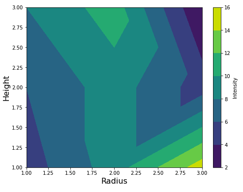
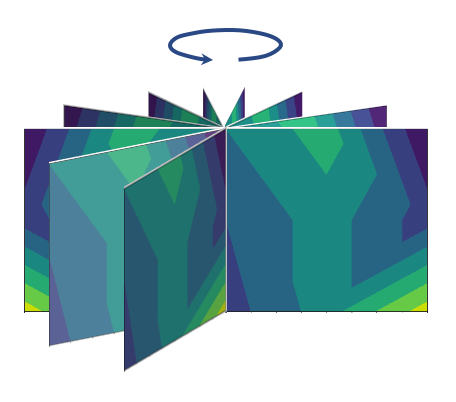
I thought you want to create a lot of pairs of filled contour plots. In each pair, the two plots are symmetric about the z axis. Here I give a matlab script:

clc
close all
clear all

sign = [-1, 1];
x = [1, 1, 1, 2, 2, 2, 3, 3, 3];
z = [1, 2, 3, 1, 2, 3, 1, 2, 3];
intensity = [5, 6, 8, 9, 9, 11, 15, 5, 2];

for i = 1:2
    x_i = x .* sign(i);
    z_i = z;
    intensity_i = intensity;

    X_I = [1:0.2:3] .* sign(i);
    Z_I = [1:0.2:3];

    [X_T, Z_T] = meshgrid(X_I, Z_I);

    intensity_T = griddata(x_i, z_i, intensity, ...
        X_T, Z_T);

    Pnts = [X_T(:), zeros(size(X_T(:))), Z_T(:)];
    T = delaunay([X_T(:), Z_T(:)]);

    patch('Vertices', Pnts, ...
        'Faces', T, ...
        'FaceVertexCData', intensity_T(:), ...
        'FaceColor', 'interp', ...
        'EdgeAlpha', 0.0, ...
        'facealpha', 1); colorbar; hold on
end

plot3([0, 0], [0, 0], [1, 3], 'k-'); hold on
text(0, 0, 3.1, 'z axis'); hold on
xlabel('x');
ylabel('y');
zlabel('z');
view(3)

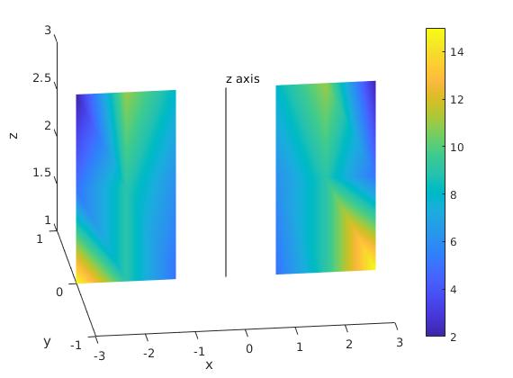
The result is below:

I only show one pair here. In the above code, I set all the y coordinates to zero, and thus, only x and z are used. The for-loop means two plot, one is in x < 0 and another is in x > 0. Then, I use meshgrid and griddata, which are kind of interpolation. Finally, I show the plot by patch command, with a triangulation created by delaunay as well as the intensity values on nodes.

I am not sure why the pair of plots looks like not symmetric. Maybe the reason is the griddata command.

---UPDATE 1---

Now, I understood your purpose: you have had some existing datasets on some planes and you wanted to interpolate more data on other planes.

Similarly, you can use griddata in matlab to do interpolation.

A matlab exmaple is below:

clc
close all
clear all

spacing_degree = 45;
range_degree = [0, 360 - spacing_degree];
NUM_plots = 360 / spacing_degree;

Pnt_3D = cell(NUM_plots, 1);
T_3D = cell(NUM_plots, 1);
Intensity_3D = cell(NUM_plots, 1);

Pnt_3D_existing = [];
Intensity_3D_existing = [];

for i = 0:spacing_degree:315

    [X Z] = meshgrid([0:0.5:2], [-1:0.5:1]);

    Pnts = [X(:), zeros(size(X(:))), Z(:)];

    if (i ~= 0)
        Pnts(:, :) = Quaternion_Rotation(i, 0, 0, 1, ...
            Pnts(:, 1), Pnts(:, 2), Pnts(:, 3));
    end

    T = delaunay(X(:), Z(:));

    Pnt_3D{i / spacing_degree + 1} = Pnts;
    T_3D{i / spacing_degree + 1} = T;

    % supposed that intensity values on xz and yz planes are known
    % I will generate some random data to represent these known data
    if (i == 0 || i == 90 || i == 180 || i == 270)

        if (i == 0 || i == 90)
            Intensity_3D{i / spacing_degree + 1} = ones(size(Pnts, 1), 1) .* ((i / spacing_degree + 1) .* 20) .* rand(size(Pnts, 1), 1);
        else
            % make symmetric data
            Intensity_3D{i / spacing_degree + 1} = Intensity_3D{(i - 180) / spacing_degree + 1};
        end

        Pnt_3D_existing = [Pnt_3D_existing; Pnts];
        Intensity_3D_existing = [Intensity_3D_existing;
                            Intensity_3D{i / spacing_degree + 1}];

    else
        Intensity_3D{i / spacing_degree + 1} = ones(size(Pnts, 1), 1) .* -20;
    end

end

% now we finished generate existing data on xz and yz plane
% and, data on other planes are all -20!
figure(1)
title('Existing data')
xlabel('x')
ylabel('y')
zlabel('z'); hold on

for i = 0:spacing_degree:315
    patch('Vertices', Pnt_3D{i / spacing_degree + 1}, ...
        'Faces', T_3D{i / spacing_degree + 1}, ...
        'FaceVertexCData', Intensity_3D{i / spacing_degree + 1}, ...
        'FaceColor', 'interp', ...
        'EdgeAlpha', 0.2, ...
        'facealpha', 1); hold on;
end

view(3); colorbar

% now let us interpolate data on other planes

for i = [45, 135]

    if (i == 45 || i == 135)

        Intensity_TT = griddata(Pnt_3D_existing(:, 1), Pnt_3D_existing(:, 2), Pnt_3D_existing(:, 3), Intensity_3D_existing(:, 1), ...
            Pnt_3D{i / spacing_degree + 1}(:, 1), Pnt_3D{i / spacing_degree + 1}(:, 2), Pnt_3D{i / spacing_degree + 1}(:, 3), 'nearest');

        Intensity_3D{i / spacing_degree + 1} = Intensity_TT;
        Intensity_3D{(i + 180) / spacing_degree + 1} = Intensity_TT;

        Pnt_3D_existing = [Pnt_3D_existing; Pnt_3D{i / spacing_degree + 1}; Pnt_3D{(i + 180) / spacing_degree + 1}];
        Intensity_3D_existing = [Intensity_3D_existing;
                            Intensity_TT; Intensity_TT];

    end

end

figure(2)
title('Existing data and interpolating data')
xlabel('x')
ylabel('y')
zlabel('z'); hold on

for i = 0:spacing_degree:315
    patch('Vertices', Pnt_3D{i / spacing_degree + 1}, ...
        'Faces', T_3D{i / spacing_degree + 1}, ...
        'FaceVertexCData', Intensity_3D{i / spacing_degree + 1}, ...
        'FaceColor', 'interp', ...
        'EdgeAlpha', 0.2, ...
        'facealpha', 1); hold on;
end

view(3); colorbar

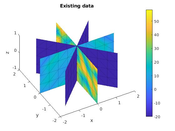
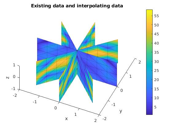
In the above code, I generated random data on xz and yz plane to represent the existing dataset, and then interpolated more data on other planes. Note that the rotation function Quaternion_Rotation is a self-defined function. If the code is helpful, I can give you that function.

Results are below:

Unknown data are all -20! Then the interpolating result is below:

Hope that the results are what you want to achieve.