Solving IVP backward in time via python

Question

I'm having difficulty solving an initial value problem (IVP) in Python backwards in time. The code is at the end of this post.

First, please let me state my simplified problem.

The forward IVP is defined as the following $$\left\{ \begin{array}{cl} u'(t)=-21 u + e^{-t}, & \ t\in[0,2] \\ u(0)=1 & \end{array} \right. $$

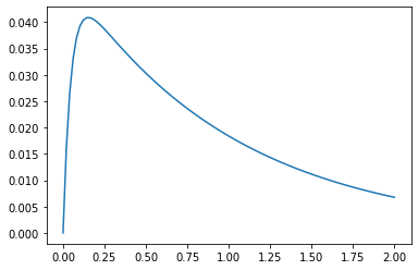
The picture below is the solution obtained by using solve_ivp package of scipy.integrate.

Up until this point, everything has gone as expected.

Now, I'd like to see if solve_ivp can solve general ODEs backward in time. For the above ODE, it should be solved from $t=2$ to $t=0$ by starting with $u(2)\approx0.00676677$.

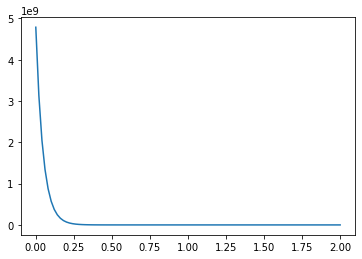
However, the backward in time solution I got was exploding

Theoretically, the forward and backward ODE should lead to the same solution (regardless numerical errors). So I'm quite confused with the result I got here.

I've testified with different drift terms, tolerance, and solvers. In some cases, numerical forward and backward solutions coincided but in most cases, they didn't.

I guess it may due to the ODEs are "stiff" but I have no clues how to fix the problem...

Below, I provide my code to this particular question.

import numpy as np
import matplotlib.pyplot as plt
from scipy.integrate import solve_ivp

#define the drift function of ode
def f(t, u):
    drift = -21 * u + np.exp(-t)
    return drift

#define hyperparameters
ti = 0.
tf = 2.
N = 100
tol = 1e-8
time = np.linspace(ti, tf, N)

#solve forward in time
sol = solve_ivp(f, [ti, tf], [0.0], method='RK45', t_eval=time, atol=tol, rtol=tol, 
      dense_output=True)
#plot forward solution
plt.plot(time, sol.y[0])
print("sol.y[0]:", sol.y[0])

#solve backward in time
sol_f = solve_ivp(f, [tf, ti], [sol.y[0][-1]], method='RK45', t_eval=time[::-1], 
        atol=tol, rtol=tol, dense_output=True)
#plot backward solution
plt.plot(time, sol_f.y[0][::-1])
print("reverse:", sol_f.y[0][::-1])

Answer 1

The error magnification factor is $e^{42}=1.739274941520501\cdot10^{+18}$. You are allowing an absolute error of $10^{-8}$ in the forward integration. Thus it is not astonishing to get an error n the size of $10^{-8+18}=10^{10}$ in the backward integration.

---

In more detail: Your DE has a boundary layer. It has an asymptotic solution at $u=\frac1{21}e^{-t}$ and a spring-like mechanism that forces any other solution to rapidly converge toward this asymptotic solution, halving the distance with time step $0.03$. In a crude Taylor interpretation, close to the asymptote the DE reads as $u(t+\frac1{21})=\frac1{21}e^{-t}\iff u(t)=\frac1{21}e^{-t+\frac1{21}}$, so the exact solution will be above the asymptote if the error tolerances are smaller $10^{-3}$.

As this is a moving equilibrium, the allowed error tolerances will be actually realized, as the step size controller detects the boundary of the stability region via the error estimates. Solutions that start far apart can become close enough in their time evolution that their distance is below the absolute tolerance and then become numerically indistinguishable.

Integrating backwards it becomes apparently random what path they follow, especially as the time steps in the backward integration are not the same as in the forward iteration. Even in fixed step methods the method step error will be different in the backward iteration, it can even have the opposite direction, increasing the round-trip error instead of (partially) erasing it.

The break-out of the tolerance bubble around the shadow of the asymptote will happen very shortly at the start of the backward integration, the distance again doubling with time step $0.03$ and with only a weak memory of where the forward integration started. If the divergence is upward or downward mainly depends on the numerical method, as said above.

Answer 2

Consider an ODE of the form:

$$d_t u(t) = \alpha u(t) + b(t), \quad b(t) = \exp(t\beta ).$$

By using an integrating factor of $\exp(-t\alpha)$ you can get the solution:

\begin{align} u(t) &= \exp(t\alpha)u(0) + \int_{0}^t\exp((t-s)\alpha)b(s)\,ds \\ &= \exp(t\alpha)u(0) + \exp(t\alpha)\int_{0}^t\exp((\beta-\alpha)s)\,ds. \end{align}

Set $\gamma = \beta-\alpha$, then if $\gamma = 0$ the solution is:

\begin{equation} u(t) = \exp(t\alpha)u(0) + \exp(t\alpha)\int_{0}^t\,ds = \exp(t\alpha)(u(0) + |t|) \end{equation}

Now let $\gamma\ne 0$, then:

\begin{align} \int_0^t\exp(\gamma s)\,ds &= \int_0^t\sum_{k=0}^{\infty}\frac{ s^k\gamma^k}{k!}\,ds = \operatorname{sign}(t)\sum_{k=0}^{\infty}\frac{t^{k+1}\gamma^k}{(k+1)!} \\ &=\operatorname{sign}(t)\gamma^{-1}\gamma\sum_{k=0}^{\infty}\frac{t^{k+1}\gamma^k}{(k+1)!} = \operatorname{sign}(t)\gamma^{-1}\sum_{k=1}^{\infty}\frac{t^k\gamma^k}{k!} \\ &= \operatorname{sign}(t)\gamma^{-1}(\exp(t\gamma)-1). \end{align}

Then if I didn't mess up something, the solution is: $$u(t) = \exp(t\alpha)u(0) +\operatorname{sign}(t)\frac{\exp(t\beta) - \exp(t\alpha)}{\beta - \alpha}.$$

Note that in the limit $\beta \to \alpha$ the second term becomes $\exp(t\alpha)|t|$, so it is consistent with the $\gamma = 0$ case. You don't need to do any time-stepping now, and you can analyze the numerical errors you can get in this expression. You can also use this to check against your numerical solutions, but either will break for a nasty combination of parameters, it's just the time-stepping would probably break earlier. As mentioned in the other answer, your problem is unstable in the backwards direction - things grow exponentially, and your error tends to blow up.