1-D incompressible unsteady Couette Flow Explicit finite differece CFD

Question

I am currently following J.Anderson Jr.'s CFD with basic application and I came into some troubles while coding for my very first CFD problem. As the title suggests I am solving an incompressible Couette flow using an explicit finite difference approach. How can I increase the steps without it blowing up? I tried to change the delta_t but it does not go any greater than what I've prescribed in the code without it going haywire any advice will be appreciated. Oh and the B.c for the upper plate is 2 unit/t

Here's the governing equation. After nondimensionalizing

And using second order central difference

The stability criterion for parabolic equation like this is:

So here's the code I have written for the central difference method referencing 12 steps to CFD by Lorena Barb

import numpy as np
from matplotlib import pyplot as py
D=1
N=21
Rey=5000
dy=D/(N-1)
dt=Rey*(dy)**2

u= np.zeros(N)
un=np.zeros(N)
un[20]=2
u[20]=2
for n in range(N-1):
    un = u.copy()
    for i in range(1, N-1):
       u[i] = un[i] + dt/Rey/dy**2 * (un[i+1] - 2 * un[i] + un[i-1])


py.plot(u/2, np.linspace(0, 2, N)/2);

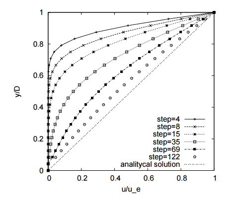
This is the graph I get

The solution graph is

I realized where I went wrong... my matrix was all messed up I was using forward time central space scheme and I did not account for my time only my space... anyway this seems to work fine

import numpy as np
from matplotlib import pyplot as plt

y_max=1
t_max=1
N=101
Rey=5
dy=y_max/(N-1)
dt=0.5*Rey*(dy)**2
u0=2

def Couette_Flow(dt,dy,y_max,t_max,u0,Rey):
    c=dt/Rey/dy**2
    y=np.arange(0, y_max+dy,dy)
    t=np.arange(0, t_max+dt,dt)
    r=len(y)
    s=len(t)
    u=np.zeros([s,r])
    u[:,0]=u0     
    for n in range(0,s-1):
         for j in range(1, r-1):
             u[n+1,j] = u[n,j] + c*(u[n,j+1]-2*u[n,j]+u[n,j-1])
    return y,u,r,s




y,u,r,s = Couette_Flow(dt,dy,y_max,t_max,u0,Rey)

This is not perfect still though I think the fact that I nondimensionalized my equation is messing with my solution, but nonetheless for small value of reynolds number it seems to generate the graph I want.

Answer 1

The answer is that you cannot increase the time step past the limit: $$ \Delta t < \frac{1}{2Re} \Delta y^2$$ This is because you are using an explicit scheme. Explicit scheme have a stability condition, which requires that the amplification factor of the whole scheme be below 1 in order to ensure stability of the scheme. In this case, this leads to the criterion you have on $\Delta t$. If you wish to use a larger time step, you need to use an implicit scheme. This will lead to the resolution of a linear system of equations.