4
$\begingroup$

I'm interested in finding the roots of the following equation:

$\tan(x) = \frac{2x}{x^2-1}$.

It is easily seen that 0 is a root and the roots are symmetric w.r.t. 0.

I wonder if an analytical solution is known or how can I find, say, 1000 roots numerically with increasing magnitudes ? I've tried Matlab built-in functions but failed.

$\endgroup$
1
  • 2
    $\begingroup$ Transcendental equations have in general no closed form solution. Finding "1000 roots" is not such a good approach. You usually try to find roots in a certain interval. $\endgroup$ Commented Jul 5, 2017 at 4:23

3 Answers 3

5
$\begingroup$

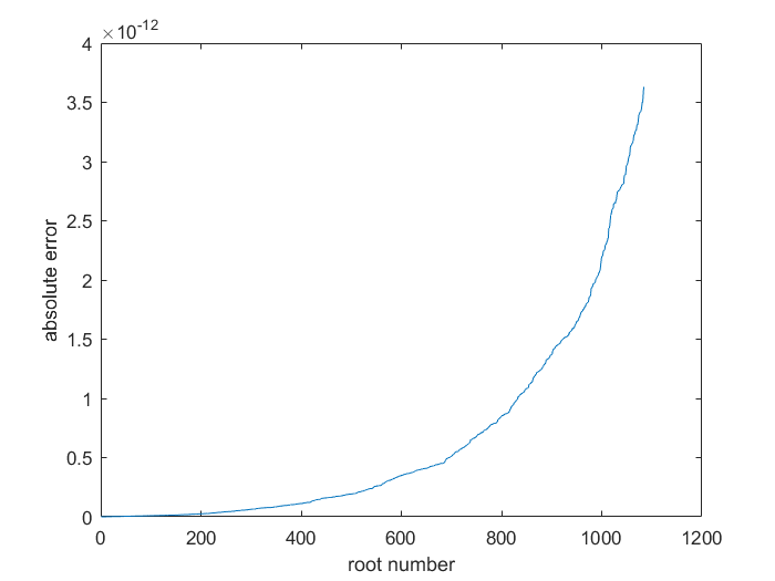
Here is a simple (Matlab) Newton method as a first attempt to help get started. It finds 1087 roots with error below $10^{-11}$.

f  = @(x) ((2*x)./(x.^2-1)) - tan(x);
fp = @(x)-tan(x).^2+2.0./(x.^2-1.0)-x.^2.*1.0./(x.^2-1.0).^2.*4.0-1.0;

x0 = 0;

for jj = 1 : 1200 %number of iterations to find some roots
    x0 = x0 + (jj-1)*(jj/10^4);  %take previous guess and increment

    for newton = 1 : 20 %number of newton steps
       x0 = x0 - f(x0)/fp(x0); 
    end
    ROOTS(jj,1)  = x0; 
    ERROR(jj,1)  = abs(f(x0));  %check that we really found a root

end

ROOTS = unique(ROOTS);  %roots may be duplicate
ERROR = unique(ERROR);  %

length(ROOTS) %number of roots we actually found

ROOTS(1:10)
ERROR(1:10)

plot(abs(ERROR))
xlabel('root number')
ylabel('absolute error')

enter image description here

Some sample roots:

Root number    |    Root value 
    300            2340.487381447216
    301            2356.195339018351
    302            2371.903296664941
    303            2387.611254385495
    304            2406.460803745755
    305            2425.310353208004
    306            2444.159902769882
    307            2463.009452429101
    308            2481.859002183444
    309            2500.708552030761
    310            2519.558101968962
    311            2538.407651996025
    312            2557.257202109985
    313            2576.106752308934
    314            2594.956302591019
    315            2613.805852954442
    316            2632.655403397457
    317            2651.504953918365
    318            2670.354504515517
    319            2689.204055187311
    320            2708.053605932186
    321            2726.903156748628
    322            2745.752707635163
    323            2764.602258590357
    324            2783.451809612815
    325            2802.301360701180
    326            2821.150911854131
    327            2840.000463070381
    328            2858.850014348680

Another option to try numerically in Matlab is the Chebfun package. It is based off the usage of orthogonal polynomials and the root finding is done by obtaining eigenvalues of the corresponding companion matrix.

$\endgroup$
2
  • $\begingroup$ Thanks a lot. Do you have any explanation on the choice of increment ? $\endgroup$
    – booksee
    Commented Jul 5, 2017 at 7:01
  • 1
    $\begingroup$ Plotting the transcendental equation and using trial/error. I first started with an arbitrary increment (like $x_0=x_0+10$). Looking at the first 5 roots or so I noticed that the difference between consecutive roots was almost some multiple of $\pi$. You could replace $x_0=x_0+(jj−1)∗(jj/10^4)$ with $x_0=x_0+(jj−1)∗\pi|$ for instance $\endgroup$
    – user107904
    Commented Jul 5, 2017 at 8:23
3
$\begingroup$

As this is a transcendent equation, finding all roots is not an option. You cannot (in general) find an expression that gives a closed-form for the roots of the equation. So you need to do some analysis first. Plotting the function, or plotting the left-hand-side and right-hand-side of the equation (and hence, the intersections of both curves are the roots) will give you some hints on how to tackle the problem. I define the LHS as $\tan(x)$ and the RHS as $\frac{2x}{x^{2}-1}$.
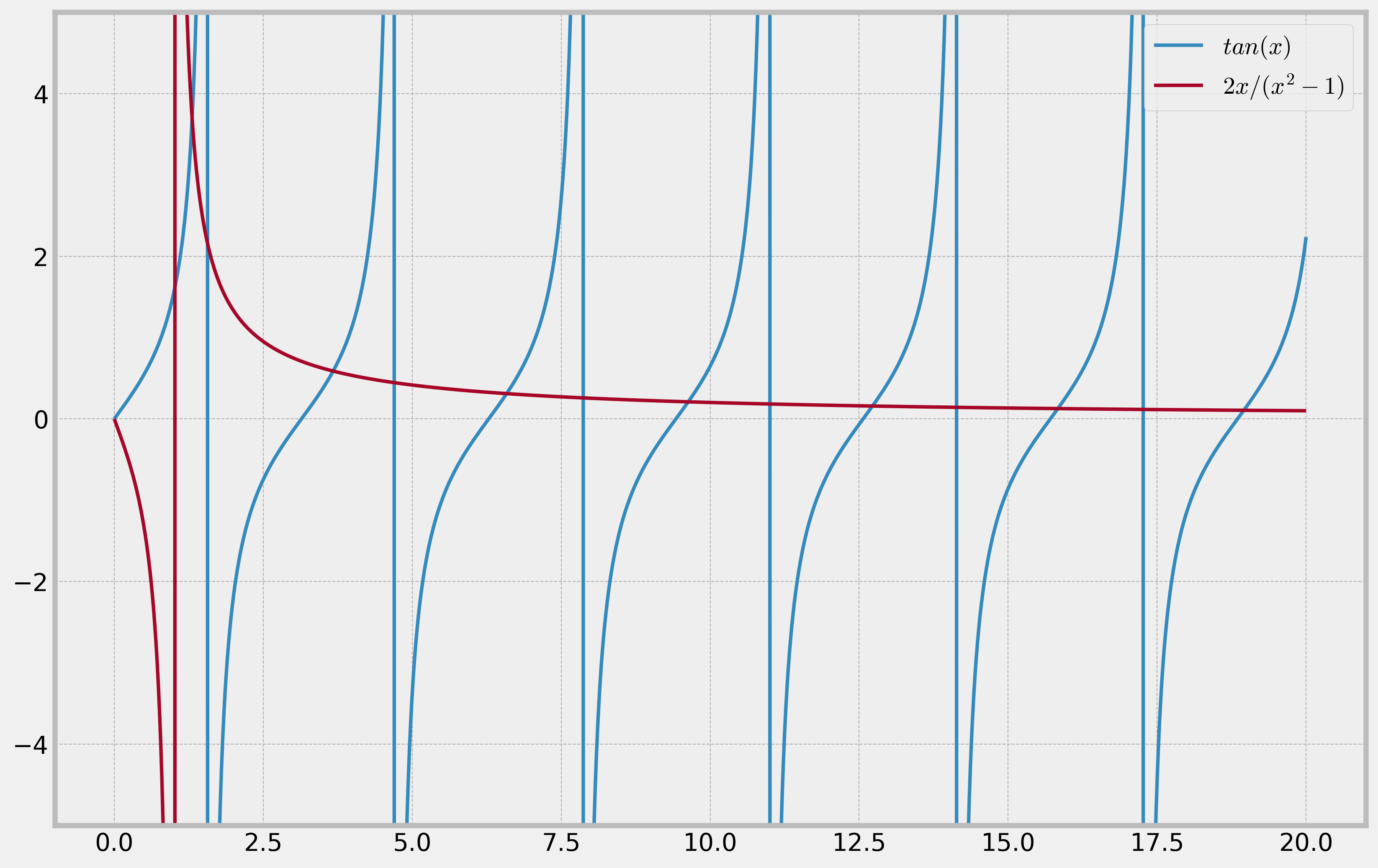
Plot of LHS and RHS

What you can observe is the following:

  • Since both LHS and RHS are (anti-)symmetric around $x=0$, you only need to consider the positive $x$ domain.
  • There is no root in the interval $[0,1[$ ($x=1$ being the location of the pole of the RHS function).
  • There is a root in the interval $[1,\frac{\pi}{2}]$.
  • Since the function of the RHS is monotonically decreasing for $x > 1$, there will be a single root in each interval $[(2k-1)\frac{\pi}{2},(2k+1)\frac{\pi}{2}]$ for $k=1,2,3, \ldots$.
  • You can see that the RHS function goes to zero for $x\to\infty$. This implies that for larger $x$, the solutions will convergence to the zero crossings of the tangent function (i.e. $r_{l} \approx (l+1)\pi$, where $r_{l}$ is the $l$'-th root. You could use these estimates as initial guess for an iterative method.

So what will be the strategy to find (not all, but an arbitrary number) of roots? You use an iterative solving method in each interval. Now you have the choice between a plethora of methods but two methods seem very appropriate:

  • Since you have a very good estimate for the root (a good initial guess), you could use Newton-Raphson. But then you need to calculate the derivative (in this case, you could do it analytically).
  • Since each root is known to be in an interval, you could use the derivative-free method of Dekker-Brent. Just make sure that you don't use the strict boundaries for each interval, because they are poles of the tangent function and Dekker-Brent will not know how to handle that. Add some margin to the initial interval.

Using the Python code below, I can find the first $N$ roots using this approach. A plot for the interval [200,300] is given as an example. Since I'm lazy and didn't want to calculate the derivative, I chose the Dekker-Brent option (where I asked for a relative tolerance of $1e-14$. For what it's worth, the first 1000 roots took me 10 ms on an Intel i5 laptop. Of course, you can validate the results by calculating the residues (the function value in each calculated root).

enter image description here

Python code:

import numpy as np
import matplotlib.pyplot as plt
from scipy.optimize import brentq

plt.figure(figsize=(12,8))
plt.style.use('bmh')
x = np.linspace(0,20,1002)
plt.ylim(-5,5)
plt.plot(x,np.tan(x),label='$tan(x)$')
plt.plot(x,2*x/(x*x-1),label='$2x/(x^2-1)$')
plt.legend(loc=1)
plt.savefig('fun.png',dpi=300,bbox_inches = 'tight')

def f(x):
    # The function
    return np.tan(x)-2*x/(x*x-1)


def roots(N):
    # Find N roots of the equation

    #Allocate space
    roots = np.zeros(N)

    #Margin to stay away from poles
    margin = 1e-8

    #First root
    roots[0] = brentq(f, 1.0 + margin, np.pi/2 - margin, rtol=1e-14)

    #Subsequent N-1 roots
    for i in range(1,N):
        left = (2*i - 1)*np.pi/2
        right = (2*i + 1)*np.pi/2
        roots[i] = brentq(f, left + margin, right - margin, rtol = 1e-14)

    return roots 

result = roots(1000)

left = 200
right = 300

plt.figure(figsize=(24,8))
plt.style.use('bmh')
x = np.linspace(left,right,(right-left)*101)
plt.ylim(0,2e-2)
plt.plot(x,np.tan(x),label='$tan(x)$')
plt.plot(x,2*x/(x*x-1),label='$2x/(x^2-1)$')
rts = result[result>=left]
rts = rts[rts<=right]
plt.plot(rts,np.tan(rts),'o', markersize=14, fillstyle='none', label='roots')
plt.legend(loc=1)
plt.savefig('roots1.png',dpi=300,bbox_inches = 'tight')
$\endgroup$
2
$\begingroup$

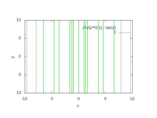
You can at least take a quick look at the zeros using gnuplot by plotting contours at zero of the equation

$$0 = \frac{2x}{x^2-1} - \tan(x)$$

set terminal png
set output "test.png"

set xlabel "x"
set ylabel "y"

set contour
set cntrparam levels discrete 0
set view map
unset surface
set isosamples 1000,1000
splot 2*x/(x**2-1) - tan(x)

Since the equation is totally independent of $y$ the solutions are lines parallel to the $y$-axis.

enter image description here

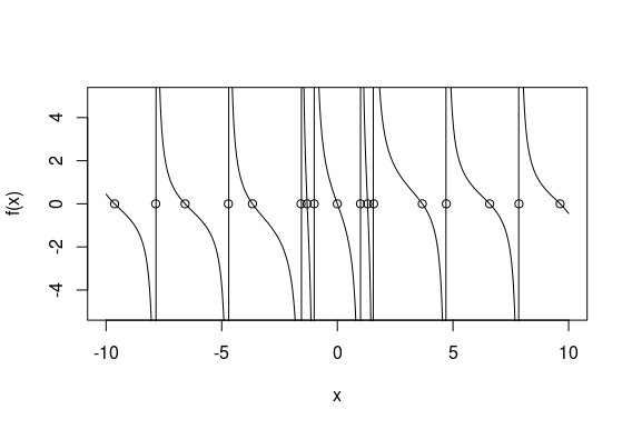
To solve the equation numerically you could use GNU R with the rootSolve package.

require("rootSolve")

f <- function(x) 2*x/(x^2-1) - tan(x)
r <- uniroot.all(f, c(-10,10))
print(r)
curve(f,-10,10,ylim=c(-5,5),n=1000)
points(r,rep(0,length(r)))

Output

 [1]  0.0000000 -9.6316827 -7.8540438 -6.5846170 -4.7124512 -3.6731884
 [7] -1.5708444 -1.3065367 -0.9999023  0.9999023  1.3065367  1.5708444
[13]  3.6731884  4.7124512  6.5846170  7.8540438  9.6316827

enter image description here

$\endgroup$
2
  • $\begingroup$ Thanks, the plots are really informative and useful for Newton method. Do you know how at most many digits can be guaranteed by the rootSolve package ? What about 10 digits ? $\endgroup$
    – booksee
    Commented Jul 5, 2017 at 7:07
  • $\begingroup$ @booksee All numbers are given in machine precision, which is 16 digits (I think). The numbers being cut off is just a consequence of formatting. $\endgroup$ Commented Jul 5, 2017 at 22:04

Your Answer

By clicking “Post Your Answer”, you agree to our terms of service and acknowledge you have read our privacy policy.

Not the answer you're looking for? Browse other questions tagged or ask your own question.