Convolute a gaussian kernel with a large array of off-grid centroids without looping? (how to make "A Thousand (Gaussian) Points of Light" )

Question

For a finite object size diffraction simulator, I need to generate arrays which are the sum of thousands of instances of a Gaussian (or other) 2D kernel at centroids that will not fall in any repeatable way with respect to the grid points.

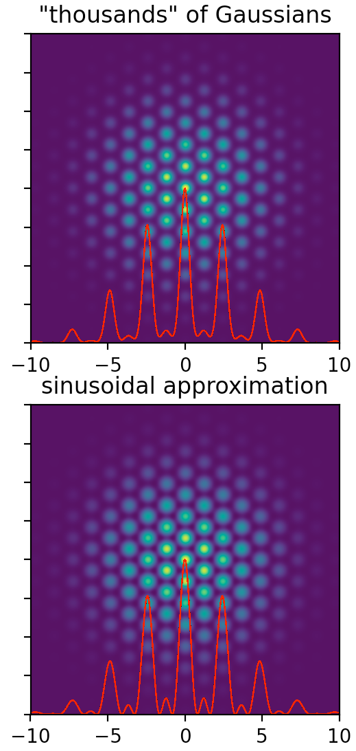
Below is a simple example with a simple hexagonal arrangement of centroids for clarity, along with a much faster analytical expression that comes close to approximating this particularly simple example, but in general the arrangement will be more complicated or even random.

import numpy as np
import matplotlib.pyplot as plt

hw = 10
N = 250
twoNp1 = 2 * N + 1
ximg, yimg = np.mgrid[-hw:hw:twoNp1 * 1j, -hw:hw:twoNp1 * 1j]
a = np.sqrt(2)
sig1 = hw/3.
sig2 = a/5.

r3o2, twopi = np.sqrt(3) / 2, 2 * np.pi

vecs = a * np.array([[1, 0], [1/2, r3o2]])
nmax = int(2 * (ximg.max()/a)) # overfill overkill
i, j = [thing.flatten() for thing in np.mgrid[-nmax:nmax+1, -nmax:nmax+1]]
keep = np.abs(i + j) <= nmax
i, j = [thing[keep, None] for thing in (i, j)]  
points = i * vecs[0] + j * vecs[1]

img = np.zeros_like(ximg)
for x, y in points:
    img += np.exp(-((x-ximg)**2 + (y-yimg)**2) / (2 * sig2**2))

# actual gaussians
img *= np.exp(-((ximg)**2 + (yimg)**2) / (2 * sig1**2))

# sinusoidal pattern
k = (twopi / (a * r3o2)) * np.array([[1, 0], [0.5, r3o2], [0.5, -r3o2]])
# that's 0, 60, -60
# try -30, 30, 90
k = (twopi / (a * r3o2)) * np.array([[r3o2, -1/2], [r3o2, 1/2], [0, 1]])

phases = [kay[0] * ximg + kay[1] * yimg for kay in k]
amplitudes = [np.cos(phase) for phase in phases]
amplitude = (1.5 + sum(amplitudes))/4.5
amplitude *= np.exp(-((ximg)**2 + (yimg)**2) / (2 * sig1**2))

if False:
    n = int((2 * hw / a)**2 + 0.5)
    randoms = hw * (2 * np.random.random((n,2)) - 1)
    rand = np.zeros_like(ximg)
    for x, y in randoms:
        rand += np.exp(-((x-ximg)**2 + (y-yimg)**2) / (2 * sig2**2))
    rand *= np.exp(-((ximg)**2 + (yimg)**2) / (2 * sig1**2))

if True:
    fig, (ax1, ax2) = plt.subplots(2, 1)
    extent = [ximg.min(), ximg.max(), yimg.min(), yimg.max()]
    one = ax1.imshow(img, origin='lower', extent=extent)
    ax1.plot(ximg, hw * (img[N] - 1), '-r', linewidth=0.5)
    ax1.set_title('"thousands" of Gaussians')
    # fig.colorbar(one, ax=ax1)
    two = ax2.imshow(amplitude, origin='lower', extent=extent)
    ax2.plot(ximg, hw * (amplitude[N] - 1), '-r', linewidth=0.5)
    ax2.set_title('sinusoidal approximation')
    # fig.colorbar(two, ax=ax2)
    plt.show()

Answer 1

The classical way to do this fast for arbitrary collections of "source" and "target" points is to use a fast multipole-type algorithm called the Fast Gauss Transform, developed by Greengard. A quick Google search turned up this Julia package implementing what the author deems an "improved" FGT: https://github.com/jwmerrill/FastGaussTransforms.jl

Based on "Improved Fast Gauss Transform," Proceedings International Conference on Computer Vision, 464 -471, C. Yang, R. Duraiswami, N.A. Gumerov, L. Davis. pdf

Answer 2

If you simply want to compute the convolution you can construct a Kernel matrix for computation with arbitrary arrangements of Gaussians that do not lie on grid points of the domain where you want to compute the convolution.

To do that one can employ an "outer sum". In python its given as done here: https://stackoverflow.com/questions/33848599/performing-outer-addition-with-numpy

In essense, one can discretize a Fredholm integral equation of the first kind into a system of linear equations to describe the convolution, i.e. in the form of $Aw=b$ and the matrix $A$ can be computed via feeding this outer sum $r_c−r_g^T$ into the Gaussian. The vector $r_c$ has all the positions in the domain you want to compute the convolution and $r_g$ is the vector that containts all central positions of the gaussians. The weight vector $w$ describes the amplitudes of the gaussians and $b$ is the resultant convolution you seek.

I rewrote your example this way in Matlab below:

%%% Positions to compute convolution
N = 150;
x = linspace(-10,10,N); 
y = linspace(-10,10,N);
[X,Y] = ndgrid(x,y);

%%% Gaussian Positions
B = [1,cosd(120);0,sind(120)];
m = 30;
d = 1.5;
[i,j] = ndgrid(-m:d:m,-m:d:m);
P = B*[i(:)';j(:)'];

%%% Compute Kernel A
Xb = X(:) - P(1,:);
Yb = Y(:) - P(2,:);
sig1 = 5;
A = exp(-(Xb.^2+Yb.^2)*sig1); 

%%% Compute Convolution
sig2 = 2e-2;
w = ones(size(A,2),1); % weight of individual gaussians
b = reshape(A*w,size(X));
% b = b.*exp(-(X.^2+Y.^2)*sig2) % if needed

%%% Plotting
imagesc(b)

Answer 3

Approximately implementing @Ron's answer in Python the key is img = (A * weights).sum(axis=2) which of course is a loop but it's done in the compiled code that numpy calls.

There may be some speed optimization possible here by adjusting the array definitions so that we can sum over a different axis and other things as well. See Code Review answers to

• Better way to calculate double-scattering diffraction using cartesian product of arrays?
• improving speed of this numpy-based diffraction calculator
• Getting hexagonal arrays of dots arranged in this spiral pattern
• and particularly Calculate electric field of a charged annulus

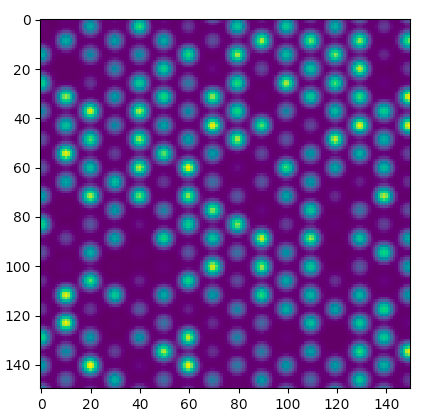
I've added random weights for demonstration purposes.

Convolute a gaussian kernel with a large array of off-grid centroids without looping?

might have been a somewhat misleading title as the problem is truly a sum over a finite number of individual centroids. The linked (and currently unanswered) question will be more of a challenge since it is a true convolution.

• How to generate the convolution of f(x, y) with a parametric function g(t), x(t), y(t) in Python? (Something better than this brute-force sum)

import numpy as np
import matplotlib.pyplot as plt

# Positions to compute convolution
N = 150
x = np.linspace(-10, 10, 150)
y = np.linspace(-10, 10, 150)
X, Y = np.meshgrid(x, y)

# Gaussian Positions
v1, v2 = np.array([[1, 0], [0.5,np.sqrt(3)/2]])
m = 30
i = np.linspace(-m, m, 40) 
I, J = [thing.flatten() for thing in np.meshgrid(i, i)]
P = v1[:, None] * I + v2[:, None] * J
keep = np.abs(I + J) <= m # makes the boundary hexagonal
P = P[:, keep]

Xb = X[..., None] - P[1]
Yb = Y[..., None] - P[0]
sig1 = 5
A = np.exp(-(Xb**2 + Yb**2) * sig1)
weights = np.random.random(len(P[1]))
img = (A * weights).sum(axis=2)